A polynomial-time algorithm for the discrete facility location problem with limited distances and capacity constraints
Isaac F. Fernandes1; Daniel Aloise1; Dario J. Aloise2; Thiago P. Jeronimo3
1 Federal University of Rio Grande do Norte; 2 State University of Rio Grande do Norte; 3 BASF
Abstract
The objective in terms of the facility location problem with limited distances is to minimize the sum of distance functions from the facility to its clients, but with a limit on each of these distances, from which the corresponding function becomes constant. The problem is applicable in situations where the service provided by the facility is insensitive after given threshold distances. In this paper, we propose a polynomial-time algorithm for the discrete version of the problem with capacity constraints regarding the number of served clients. These constraints are relevant for introducing quality measures in facility location decision processes as well as for justifying the facility creation.
Keywords: Location Theory; Limited Distances; Capacity Constraints.
1 Introduction
Location Analysis is one of the most active fields in terms of Operations Research. It deals with the decision of optimally placing facilities in order to minimize operational costs (Nickel et Puerto, 2005). Solved in several situations by intuitive methods, facility location decisions usually demand more in-depth studies. Regardless of the type of business in which the company is involved, the decisions about location are strategic and belong to the core of any management process. Furthermore, these decisions lead to long term commitments (Moreira, 2010) due to high costs involved in installing location facilities.
Each location problem depends on the interests of the organization. Thus, some companies prefer to be closer to clients (like supermarkets, hospitals or police stations), while others are attracted by the proximity to raw materials or components (such as cement factories or potteries), or even by places where the labor is plenty, well trained or cheap, depending on the type of business.
This type of problem has been subject of scientific studies for a long time. It traces back to Fermat in the 17th century, who proposed the following problem: for three given points in a plane, find a fourth one so that the sum of its distance to the three existing points is minimum. This geometrical problem was solved by Torricelli in 1647 (see more in Wesolowsky, 1993; Smith et al., 2009).
In 1909, Alfred Weber proposed a generalization for this problem. The minisum problem, also known as the Weber problem (cf. Wesolowsky, 1993; Fekete et al., 2005) is a central problem in location theory. It refers to a situation in which there exists a set of demand points and the location of a facility must be chosen such that the total sum of the weighted distances from the points to the facility is minimized. The function to be minimized is presented below:
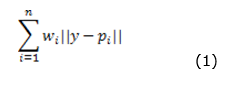
Where n is the number of client points p1, p2,..., pan in ℝ2; wi are weights and; ||.|| is the Euclidean norm. The Weber problem is convex with a non-differentiable objective function, since the facility location may coincide with a client location. Real life applications for this problem are many (e.g. Correa et al., 2004; Johnson et al., 2005; Pelegrín et al., 2006; Beresnev, 2009; Marín, 2011).
The choice of the location may have influence over the relations between the company and its clients. If the client must be physically in the process, it is unlikely that a location is acceptable if the travel time or distance between the provider and the client is large (Krajewski et al., 2009).
Particularly, for some emergency services (e.g. ambulances, police calls), the service provided by the facility has no effect after certain threshold time/distance. For example, a house on fire would be completely destroyed after a given period of time. In the case of a police call, criminals would be likely untraceable after a time limit.
This model characteristic can be approached in different ways. Evans et al. (1997) proposed a min-max model to determine the location for these types of emergency units. The model has the objective of locating a facility among a group of candidates, such that the distance to the farther client is minimized. Drezner et al. (1991) proposed a variation of the Weber problem to model location problems in which the service provided by the facility is insensitive after a threshold distance (directly related to a maximum time limit). To illustrate their model, let us use an example provided by Drezner et al. (1991) to locate a fire station. In this context, each property has a limit distance after which the service provided by the fireman would be useless, and the property would be completely destroyed. A certain damage occurs in a property located in pi for i = 1,…, n at a null distance from the fire station (located at y ∈ ℝ2), linearly increasing up to a distance λi, where the damage is 100%. By denoting d(pi, y) the distance between the point pi and the facility located at y, and Ω the proportion of damage at zero distance, the proportion of damage in pi is given by Ω + (1 – Ω) d(pi, y) / λi in the case d(pi, y) < λi, and 1 otherwise. The corresponding facility location problem is then expressed as:
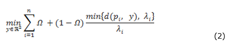
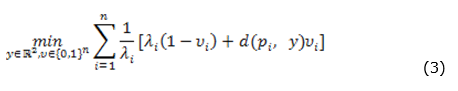
The first term of the summation is constant and (1 - Ω) is irrelevant to the second term. By introducing binary variables υi that select between d(pi, y) and λi to the summation of the objective function, we have the minimization problem defined in (3).
Fernandes et al. (2011) extended the model of Drezner et al. (1991) by adding capacity constraints to the service provided by the facility. In some real applications, during the operation of a facility, there are a maximum number of clients who can be served without affecting the service quality. In other situations, it is necessary to add to the model a minimum limit of users that would justify the existence of the facility.
The structure of the paper is as follows. The discrete facility location problem with limited distances and capacity constraints is mathematically formulated in the next section. In the following, our solution algorithm is described and a formal demonstration of its optimality is presented. After that, we report our test results, referring to the efficiency and effectiveness of the algorithm. Finally, conclusions are given in the last section.
2 Mathematical definition of the problem
Let us define d(pi, y) as the distance between point pi and the facility y located in ℝ2. Given n service points in the plane p1, p2,..., pn with limited distances λi > 0 and weights wi ≥ 0 for i = 1,..., n, the discrete limited distance in terms of the minisum problem with capacity constraints may be expressed by:
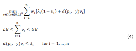
The first set of constraints defines bounds LB and UB in the number of variables Ui that can be equal to 1. The second set of constraints assures that Ui can be equal to 1 only if the distance between pi and the facility located at y is inferior (or equal) to the limit distance λi. This avoids the attribution Ui = 1 only to satisfy the constraint  . The objective function of (4) and its feasible set is non-convex, which demands more sophisticated solution methods. In this model the variable y may assume a value from a discrete finite set of values Y.
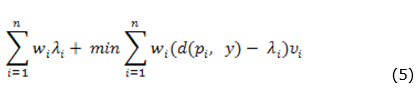
The objective function (4) may still be rewritten by removing its constant terms. It is then expressed as:
Fernandes et al. (2011) approached the continuous version of the problem. The only difference between the continuous and discrete version lies in the fact that the facility location y is constrained to be in ℝ2, instead of within a finite set Y  ℝ2. The authors propose a global optimization algorithm for the problem based on a decomposition that, initially, selects for evaluation only the sub regions of the plane that may contain the optimal solution y*. Next, each subproblem is convexified and then solved by convex optimization solvers.
Discrete location models are very common in real applications where there are often a finite number of potential places where the facility can be installed. The p-median problem (cf. Galvão, 1980; Mladenović et al., 2007) is a popular example of a discrete facility location model.
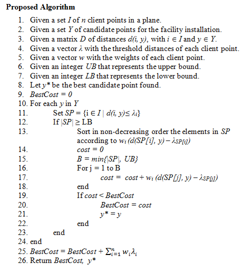
Proposed polynomial time algorithm
Problem (4) has a smaller complexity if compared to its continuous version, since the number of potential candidates is already known beforehand in the plane. The pseudo-code of the algorithm proposed here to the problem is presented in Figure 1. From lines 1 to 7, the variables that configure an instance for the problem are created, while lines 8 and 9 create two variables to store the best solution y* with its corresponding cost (BestCost). The main loop in lines 10-24 calculates, in each iteration, the facility installation cost for a candidate place, and selects the best alternative.
For a candidate point y, line 11 assigns to the set SP all the client points that can be served if the facility is installed in y, according to the limited distance constraint. If the cardinality of SP is superior to the lower bound LB (logical test at line 12), the elements from SP are sorted in non-decreasing order according to the difference 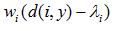 (observe that these values are negative by SP definition). The current solution cost is initialized at line 14. In line 15, B is defined as the amount of client points that would be served by the candidate point – either the regular quantity served or maximum UB, in case |SP| is superior to UB. The loop in lines 16 to 18 is iterated until all the points in B are considered. The best solution is updated in lines 19-22 if the investigated solution at the current iteration is better. Finally, the best solution is returned in line 26, with cost corrected through the addition of the constant term
  in line 25.
Figure 1. Polynomial-time algorithm proposed to the optimization of problem (4).
The proposed algorithm is polynomial, and its complexity is analyzed by observing its structure. The loop in lines 10-24 is executed for each location that is candidate for facility installation (O(|Y|)). The SP set construction at line 11 takes O(|I|) time, since all client points are evaluated for their inclusion in SP. The sorting operation in line 13 for the elements in SP has complexity O(|I| * Log (|I|)), and it is the most expensive operation for the main loop. Hence, the final complexity of the algorithm is O(|Y| * |I| * Log(|I|)). The optimality of the algorithm is assured by the proof below.
Proposition 1: The proposed algorithm finds the optimal solution for the discrete single facility location problem with limited distances and capacity constraints.
Proof: Let us assume y* as the optimal place to the installation of the facility.
The algorithm selects the first B elements of SP where B = min{∣SP∣, UB}. These elements i  SP are sorted increasingly according to wi (d(i, y*) – λi) ≤ 0.
Let us assume an optimal solution v, which corresponds to the points served by y, respecting . We have vi* = 1, if the facility in y* counts the term wid(i, y*) in the objective function and vi* = 0 if it counts wiλi.
Let us denote V = {i | vi* = 1}. Let’s analyze two situations:
a) ∣V∣ < B.
If B = |SP| or B = UB, we can take an element i' ∈ SP and i' ∉ V so that vi'* = 1. This way, we obtain a better solution than the previously assumed best solution (a contradiction).
b) ∣V∣ > B.
If B = UB and ∣V∣ > B, the solution assumed as the best is infeasible. Otherwise, if B = ∣SP∣, there is an element i' in V that doesn’t belong to SP. Thus, this element may be removed from the solution (vi'* = 0) in order to obtain a better solution than v* (contradiction).
So, ∣V∣ = B. Yet, we still need to prove that the elements in V correspond to the first B elements in SP. Let us suppose that this is not true: there is an element i1 among the first B elements from SP that is not in V. Without loss of generality, we also assume wi (d(i, y*) – λi) ≠ wj (d(j, y*) – λj),  i,j ∈ I. Since ∣V∣ = B, there is an element i2 in V that is not among the B first elements from SP. Therefore, V is not optimal, because we can do vi1* = 1 and vi2* = 0, and consequently, the solution cost of v* is improved (contradiction).
Hence, the algorithm proposed in Figure 1 finds the optimal solution for the discrete single facility location problem with limited distances and capacity constraints.
3 Computational tests
To evaluate the performance of the algorithm proposed, two sets of experiments were devised. The first one tests the efficiency of the algorithm and its computational limits, while the second set tests the accuracy and efficacy of the algorithm to provide an approximation to the continuous version of the problem.
The algorithm was run in an Intel Core 2 Duo E4500 platform with 2.20 GHz and 2 Gb of RAM memory. The algorithm was implemented in C++ and compiled by Dev-C++.
First set of experiments: accessing algorithm’s performance
In this set of tests, we tried to detail the performance of the algorithm under different possible scenarios, which may help the decision maker to define its application and usability for real-world problems. These tests were designed to investigate the influence of: (i) the threshold distance value, (ii) the lower and upper bounds: LB and UB, and (iii) the number of candidate/client points for facility location over algorithm performance.
Problem instances were artificially generated from a uniform distribution in the unit square. The threshold distances scenarios were created with 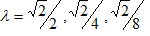 , where
  is the diagonal of the unit square. In this set of experiments, all generated points are candidate for installing the facility.
The instances are listed in Table 1. In the first column it is shown the number of points in each instance. In the second column the threshold distance for each instance is given, and in the next two columns the capacity constraints values LB and UB are defined. The last two columns report CPU times (in seconds) and the obtained cost, respectively.
Table 1. Results for the first set of experiments
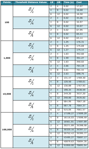
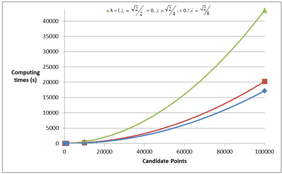
In Table 1, we note that variation in the threshold distance value directly affects the computing times. For instances with the same number of points, as well as the same lower and upper bounds, increasing the threshold distances is likely to increase the cardinality of SP. Indeed, candidate points may now be closer to client points, thus eventually serving more points within the allowed distance. The most expensive part of the algorithm occurs in line 12 of the algorithm, where the set SP is sorted – the bigger the set is, the longer it takes to sort. For example, in the instances with 100,000 points, including 2 and 4 as capacity constraints values, the computing time varies from 17,198.27 to 43,495.27 seconds by changing the threshold distances. CPUs time also increase as the number of candidate point for facility location augments, as shown in Figure 2 for the instances with LB = 2 and UB = 4.
Figure 2. Computing times for instances with LB = 2 and UB = 4 with different threshold distances. The curves are approximated by quadratic functions
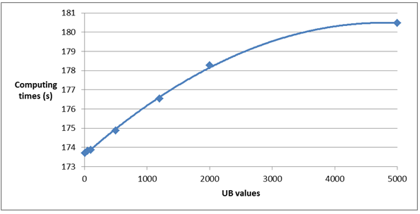
Other parameters that may affect the algorithm’s efficiency are the capacity constraint values LB and UB. Regarding the upper bound value, as UB augments, more points in SP set may have to be verified in lines 15-17 of the algorithm. Figure 3 presents increasing computing times as UB augments in the instance generated with 10,000 points, with  and LB = 2.
Figure 3. Decay in the algorithm’s efficiency due to an increase in the upper bound value in the instance with 10,000 points,  and LB = 2. The curve is approximated by a quadratic function.
Lower bound values usually have a considerable impact over the algorithm performance, its intensity depending on the dispersion of the points of the instance. As larger lower bounds LB are used, the algorithm takes less time to execute them since more candidate points do not meet the condition in line 11. Figure 4 shows the computing time spent by the algorithm on solving the generated instance with 10,000 points, with  = 0.1 and UB = +∞, while varying the lower bound value LB.
Figure 4. Computing time decay caused by an increase in the lower bound value in the instance with 10,000 points, = 0.1 and UB = +∞.
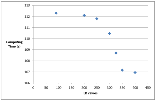
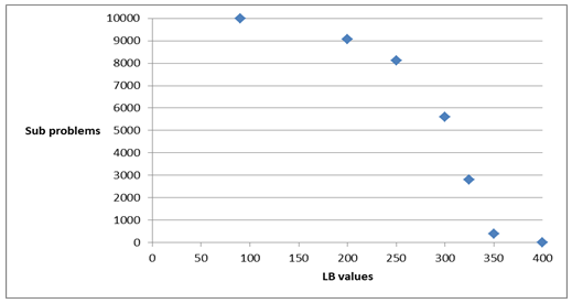
Figure 5 presents the variation in the number of subproblems for the same experiment, i.e. |SP| ≥ LB, as the lower bound value increases. We note that the number of subproblems decreases in the same rate of the graph in Figure 4. They actually have the same behaviour and show the importance of the LB parameter for the performance of the algorithm.
Figure 5. Number of subproblems solved as LB augments and UB = +∞ in the instance with 10,000 points and = 0.1.
Second set of experiments: comparison with the global optimization approach
Fernandes et al. (2011) proposed a global optimization algorithm for the continuous version of the facility location problem with limited distances and capacity constraints. In this section, we test how the algorithm, proposed here, approximates the solution of the continuous problem in the instances of Fernandes et al. (2011) when used as a grid search method.
To perform this comparison, we constructed a grid with a mesh that adjusts the precision of our approximation. The grid is bounded by the location of the most distant points, and the limited plan is divided in an equal number of cells as shown in Figure 6. The points in the intersections of the cells represent candidate points to facility location.
Figure 6. Grid for the problem divided in nine cells. The black dots represent the clients and the red ones represent candidates to facility location.
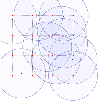
The quality of the approximation depends directly on the size of the mesh. A mesh with size g=3, has 3x3=9 cells. This value influences algorithm’s performance due to its direct relation with the number of candidate points. As g increases, more candidate points are put in Y, thus improving the quality of the approximation.
Fernandes et al. (2011) proposed 9 instances, with different numbers of client points, threshold distances and capacity constraint values. The instances can be found at http://www.gerad.ca/~aloise/publications.html. They may be divided into three groups, according to the number of clients: the first 3 have 10 client points, the next 3 have 100 and the last 3 have 1000 client points. The lower and upper values (LB) and (UB) were made constant within each group: LB= 2, UB= 4 for instances with n = 10; LB = 4, UB = 8 for instances with n = 100 and; LB = 6, UB = 12 for instances with n = 1000.
Table 2 reports the results obtained by the grid search algorithm proposed here in comparison with the results of Fernandes et al. (2011) for the continuous model. The first column presents the name of the instances. The second column shows the threshold distances of the instances, which is equal for all candidate points. The next six columns present cost results and computing time for different g values. Each cost value is reported by a ratio between the optimal solution value in the continuous model, obtained by the decomposition algorithm, and the solution value obtained by the grid search algorithm. Finally, the last two columns report the optimal solutions and CPU time spent by the decomposition algorithm of Fernandes et al. (2011) on solving the continuous model.
Table 2. Comparison of results between the grid search algorithm and the decomposition algorithm of Fernandes et al. (2011)
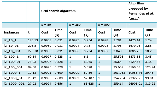
The continuous model is a relaxation of model (4) (since  ). Consequently, the solutions obtained by the grid search algorithm are always greater or equal to the solutions obtained in the decomposition algorithm of Fernandes et al. (2011). However, it is noted that, for the instances tested, the ratio between their costs was never inferior to 0.99, which attests the goodness of our approximation in the tested instances (this conclusion cannot be directly generalized for all possible instances due to the limitation of grid search global optimization algorithms – cf. Hendrix and Tóth (2010)).
Figures 7 and 8 illustrate how the grid search and decomposition algorithms are influenced by the threshold distance values in the instances with 100 and 1000 points, respectively. For both figures, we note that the grid algorithm is insensitive to (indeed this value is just slightly increased in this set of experiments), and increases its CPU time as g augments. In Figure 3, the decomposition algorithm is outperformed by the grid search algorithm, regardless of the mesh precision; however, ≥ 73.23. For the instances with 1000 points, this happens for ≥ 27.02. Furthermore, we can also conclude from the figures that the decomposition algorithm is always outperformed by grid search algorithms in the tested instances if g ≤ 50.
Figure 7. Computing time for instances with 100 points spent by the grid search algorithm for g values of 50, 250 and 500, and by the decomposition algorithm (Tdecomposition)
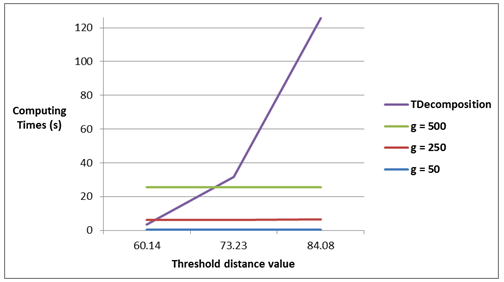
Figure 8. Computing time for instances with 1000 points spent by the grid search algorithm for g values of 50, 250 and 500, and by the decomposition algorithm (Tdecomposition)
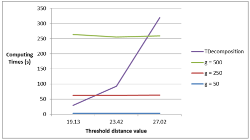
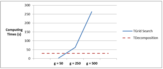
Figures 9 and 10 show the influence of the value g over the performance of the grid search algorithm in instances l2_1000_1 and l2_1000_001. The curves in the figures present CPU time spent by the grid search algorithm for different values of g. The dotted lines in both figures represent CPU time spent by the decomposition algorithm in the referred instances. As observed, the performance of the grid search algorithm deteriorates as more candidate points are searched. This deterioration is accompanied by an improvement in terms of the approximation, representing a tradeoff for the decision maker between quality and performance when using the grid search algorithm. Indeed, the decomposition algorithm is preferred when it presents a better performance than the grid search algorithm for a particular value of g (for instance, in Figure 6, for g ≥ 250).
Figure 9. CPU time for the instance l2_1000_001 spent by the grid search algorithm for g values of 50, 250 and 500, and by the decomposition algorithm (Tdecomposition)
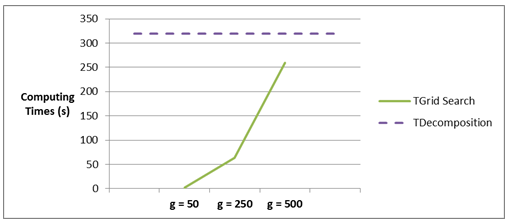
Figure 10. CPU time for the instance l2_1000_1 spent by the grid search algorithm for g values of 50, 250 and 500, and by the decomposition algorithm (Tdecomposition)
Conclusions
The introduction of capacity constraints while locating a facility in the plane with limited distances may serve to justify its installation or to describe service limitations. This work sought to analyze the single facility location problem with limited distances and capacity constraints for a finite set of candidate points. Fernandes et al. (2011) devised a global optimization decomposition method to the same model, but with the possibility of locating the facility in the continuous Euclidean plane.
In this paper, we proposed a polynomial-time algorithm to the discrete problem. The algorithm was tested for different scenarios by varying instance parameters that influence its performance, such as the number of candidate points, threshold distance values, and lower and upper bounds in the number of served points. Moreover, we compared our algorithm within a grid search framework with the decomposition algorithm of Fernandes et al. (2011). These computational experiments showed that the quality of approximation provided by the grid search algorithm in the tested instances is high, always above 99%. While the quality of the approximation can be further improved by increasing the precision of the mesh, the performance of the algorithm is compromised since its computational complexity depends directly on the number of candidate points for facility installation.
As shown by the experiments, the proposed algorithm can work with instances with thousands of demand points. It is worth mentioning that the mathematical formulation of the problem, as well as the algorithm proposed here, does not depend on the distance norm adopted; it only considers that a distance matrix is provided.
References
Beresnev, V. L. (2009) Upper bounds for objective functions of discrete competitive facility location problems. ISSN 1990-4789, Journal of Applied and Industrial Mathematics, Vol. 3, No. 4, pp. 419–432.
Bonami, P.; Lee, J. (2007) BONMIN user's manual. Technical report, IBM Corportaion.
Correa, E.S., Steiner, M.T.A., Freitas, A.A., Carnieri, C. (2004) A genetic algorithm for solving a capacitated p-median problem. Numerical Algorithms, Vol. 35, No.2-4, pp. 373-388.
Drezner, Z.; Mehrez, A.; Wesolowsky, G. (1991) The facility location problem with limited distances. Transportation Science. Vol. 25, No 03, pp. 183–187. Available: http://transci.journal.informs.org/cgi/content/abstract/25/3/183. Access: 6th December 2010.
Evans, J.R.; Anderson, D.R.; Sweeney, D.I.; Williams, T.A. (1997) Applied Production and Operations Management. 2nd Ed. St Paul, MN: West Publishing Company.
Fekete, S. P.; Mitchell, J. S. B.; Beurer, K. (2005) On the continuous Fermat-Weber problem. Operations Research, vol. 53, No. 1, pp. 61-76.
Fernandes, I.F., Aloise, D., Aloise D.J., Hansen, P., Liberti, L. (2011) On the Weber facility location problem with limited distances and side constraints. Cahiers du GERAD G-2011-18. Available at http://www.gerad.ca/~aloise/publications.html
Galvão, R.D. (1980) A dual-bounded algorithm for the p-Median problem. Operations Research, Vol. 28, No. 5, pp. 1112-1121. Hendrix, E. M. T.; Toth, B. G. (2010) Introduction to Nonlinear and Global Optimization. Springer, Cambridge.
Johnson, M. P.; Gorr. W. L.; Roehrig, S. (2005) Location of service facilities for the elderly. Annals of Operations Research, Vol. 136, No. 1, pp. 329-349.
Krajewski, L.; Ritzman, L.; Malhotra, M. (2009) Administração de Produção e Operações. 8th Ed. São Paulo: Pearson / Prentice Hall. Marín, A. (2011) The discrete facility location problem with balanced allocation of customers. European Journal of Operational Research, Vol. 210, No.1, pp. 27-38.
Mladenović, N.; Brimbergb, J.; Hansen, P.; Moreno-Pérez, J.A. (2007) The p-median problem: A survey of metaheuristic approaches. European Journal of Operational Research. Vol. 179, Issue 3, pp. 927-939.
Moreira, D.A. (2010) Administração da Produção e Operações. 2nd Ed. São Paulo: Cengage Learning.
Nickel, S.; Puerto, J. (2005) Location Theory: A Unified Approach. 1st Ed. Springer.
Pelegrín, B.; Fernández, P.; Suárez, R.; Garcia, M. D. (2006) Single facility location on a network under mill and delivered pricing. IMA Journal of Management Mathematics, Vol. 17, No. 4, pp. 373-385.
Smith, H.K.; Laporte, G.; Harper, P.R. (2009) Locational analysis: highlights of growth to maturity. Journal of the Operational Research Society, Vol. 60, No. 1, pp. 140-148.
Wesolowsky, G.O. (1993) The Weber problem: History and perspectives. Location Science, Vol. 1, No. 1, pp. 5–23.