
castrolopes.carolina@gmail.com
Pontifical Catholic University of Rio de Janeiro – PUC-Rio, Rio de Janeiro, Rio de Janeiro, Brazil.
Pontifical Catholic University of Rio de Janeiro – PUC-Rio, Rio de Janeiro, Rio de Janeiro, Brazil.
Pontifical Catholic University of Rio de Janeiro – PUC-Rio, Rio de Janeiro, Rio de Janeiro, Brazil.
Pontifical Catholic University of Rio de Janeiro – PUC-Rio, Rio de Janeiro, Rio de Janeiro, Brazil.
Goal: The objective of this article is twofold: (i) analyze the investment in a new refinery in Brazil and identify the optimal moment to invest; and (ii) model the crack spread adjusted to the Brazilian market.
Design / Methodology / Approach: The main uncertainties given by the crack spread and the foreign exchange rate were modeled as a continuous mean reversion model and geometric Brownian motion, respectively. The project was valued based on a real-option approach, including the option to postpone and the option to temporarily shut down. The first was assessed from analytical solution of the differential equation, while the latter was obtained from Monte Carlo simulation.
Results: The investment decision changes depending on the expiration date of the postponement option and the stochastic treatment of the initial investment. The temporary shutdown option increases the value of the refinery and may change the decision of postponement.
Limitations of the investigation: The crack spread was modeled based on international market because of limited availability of data from the Brazilian market. Additionally, results are dependent on the uncertainties and flexibilities modeled.
Practical implications: The analysis comprising both options is especially relevant because there are refinery projects discontinued in Brazil, and the country is an oil products’ importer.
Originality / Value: The paper contributes with an analysis in the refining industry considering the optimal moment to invest based on the interaction of two different options. Especially original is the crack spread modeling adapted to the Brazilian market.
Keywords: Investment Analysis; Real Options Theory; Stochastic Process; Refinery; Crack Spread.
The refining industry is responsible for processing petroleum and producing derivative products demanded by society. Crude oil has no use: it is the refining process that turns oil into various products, such as diesel, gasoline, aviation kerosene, bunker for ships supply and liquefied petroleum gas (LPG).
Building and operating a new refinery consists in a complex and capital-intensive project, subject to several uncertainties that affect its revenues and costs. The major source of uncertainty in the cash flow is the difference between the cost of the supply (oil price) and the value of the final products (such as diesel, gasoline, naphtha, and fuel oil) given by the price of each one in the market (Kemna, 1993; Población and Serna, 2016). While other costs can be more easily predicted, the prices of oil and derivatives are uncertain and subject to constant variations (Imai and Nakajima, 2000). This difference between the price of derivatives and oil is known in the refining industry as the crack spread.
The operation of a refinery is subject to several managerial flexibilities that represent opportunities to review future actions and decisions that depend on an uncertain future (Trigeorgis, 1993). The flexibilities and uncertainties inherent in a refinery need to be considered in the assessment of the feasibility of the investment. The discounted cash flow (DCF) approach and its main indicator, net present value (NPV), although widely used as the main criteria for investment decisions, do not value the implicit flexibilities present in projects. The real options theory, however, deals with the analysis of investment under conditions of uncertainty and emphasizes the value of managerial flexibilities in a project.
In the context of the refining industry, the option to wait to invest, the shutdown option and the option to switch inputs used or derivatives produced (switch input-output) become relevant. Other options such as abandonment and expansion can also be evaluated. The option to wait, also called option to postpone or to defer, is relevant to the investment analysis given the high amounts associated with the construction of a new refinery and the future uncertainty of return on investment, which depends on oil and derivatives prices. The shutdown option is interesting at certain moments due to the fluctuation in the price of oil and derivatives, which may lead to a reduction of the crack spread and, consequently, to the optimal choice of interrupting the refinery operation. Input-output switching options may occur when it is worthwhile to use a particular type of oil as input or to produce a different mix of products derived from refining.
Real option approaches have been used in the literature of crude oil refineries (Costa and Samanez, 2009; Imai and Nakajima, 2000; Kemna, 1993; O’Driscoll, 2016; Yi, 1997) and more recently to analyze renewable energy sources as biomass (Li et al., 2015; Sharma et al., 2013), resulting in relevant gains when compared to traditional investment analysis approaches. However, while there is a vast literature on the modeling of prices of oil and oil products alone or even on the spread of two products (Azevedo et al., 2015; Dempster et al., 2008; Pindyck, 1999, 2001), there are not many applications for modeling directly the crack spread of an oil refinery (Población and Serna, 2016; Yi, 1997). Additionally, the crack spread is usually calculated based on a proportion of refined products produced by refineries in the North American market.
Brazil is an importing country of refined products. According to Yabiko and Bone (2016), the country needs two new refineries producing around 350 thousand barrels a day until 2030 to achieve self-sufficiency in the derivatives market. Thus, considering the importance of assessing more accurately investment opportunities in crude oil refineries in Brazil, this article seeks to contribute to the literature in two ways: (i) with an analysis of the investment in an oil refinery in the country, considering the optimal moment to invest in the project; and (ii) modeling the crack spread adapted to the reality of refining in the country. The article proposes an application of the real options theory in the refining industry, evaluating the option to postpone based on a deterministic or stochastic investment; the option to temporarily shut down the refinery operation; and finally, the interaction between both options. Two uncertainty variables are modeled: the crack spread, adapted to the Brazilian market, and the foreign exchange rate, given that oil and derivative prices are defined in international markets and priced in US dollars. The use of Monte Carlo simulation facilitates the treatment of the cash flow and allows the evaluation of the proposed options.
Following Castro Lopes et al. (2020), the crude oil refinery under analysis is 85% complete. Therefore, the case with the incremental investment to finalize the project is considered, as well as the total value of the investment needed for a new refinery, in order to evaluate whether the investment decision would be different if the project had not been started yet. This article comprises five parts. The first is this introduction. Then, a literature review about real options in the refining industry is presented, followed by the methodology described in the third part of the paper. The results are discussed in the fourth part and finally the last section concludes the article.
According to Dixit and Pindyck (1994), the classic rule of investment decisions based on DCF method compares the situation of investing today with the situation of never investing assuming a scenario of expected cash flow values. Thus, the three main characteristics of the investment decision are neglected: irreversibility, optimal time to invest, and uncertainty. The real options approach allows including and evaluating decisions that managers can make over the life of a project under uncertainties that affect the cash flows.
A real option is a right, not an obligation, in a decision-making process about real assets. Uncertainties such as commodity and final product prices, demand, exchange rates, and other macroeconomic variables can affect decisions made by managers during the life of a project and impact its value. The Real Option Theory allows quantifying the value of flexibilities: the more the company's ability to adapt, the more value is added to the project (Dias, 2014).
The refining business is based on the gross margin of derivatives over the oil that is processed, that is, through the difference between the sale price of the derivatives and the purchase of the oil (crack spread), causing refiners to direct their attention to the difference between these prices, rather than the price level of each product (Clews, 2016; Yi, 1997). The crack spread is the main uncertainty of this business.
Although each refinery has its own crack spread that can be calculated from the processed oil and the produced outputs, there is a measure that represents the gross margin of a typical refinery, called 3:2:1 crack spread. The ratio 3:2:1 refers to the proportion of the derivatives produced from a certain quantity of oil: from processing three barrels of oil, two barrels of gasoline and one of diesel are typically produced (O’Driscoll, 2016). The crack spread represents the gross margin of the refinery and oil cost accounts for approximately 85% of refining operational costs, while the sale of diesel and gasoline accounts for about 80% of total revenue (Yi, 1997).
The value of the crack spread, as well as other commodities, is governed by market mechanisms, that is, supply and demand. When prices are high, commodity producers increase supply, causing a decrease in the price. Similarly, when prices are low, producers restrict the supply and consequently shortages cause increase in the price. This behavior characterizes a mean reversion process and is typical of commodity prices, a well-established fact in finance literature (Aiube, 2013). Both the spread of prices and the prices of oil derivatives are usually modeled as mean reversion models (MRM) (Costa and Samanez, 2009; Dempster et al., 2008; O’Driscoll, 2016; Vianello and Teixeira, 2012; Yi, 1997).
Considering that oil and derivatives prices are formed in international markets, the uncertainty associated with the foreign exchange rate also becomes relevant to analyze a project in Brazil. The exchange rate is generally modeled in the literature as a Geometric Brownian Motion (GBM) process (Oliveira, 2014; Teles, 2005).
For industries with similar characteristics, such as the petrochemical and biofuel refineries, in addition to relevant price fluctuations observed (Fonseca, 2008; Leiras et al., 2008), some papers propose modeling the uncertainty associated with demand, more specifically the size of the market (Sharma et al., 2013; Vianello and Teixeira, 2012), and the value of the investment (Fonseca, 2008; Vianello et al., 2014; Vianello and Teixeira, 2012). In the case of this paper, demand uncertainty becomes less relevant because Brazil is an importing country of oil products; thus, this article assumes that the refinery under analysis has the capacity to substitute imports. Yabiko and Bone (2016) conclude that Brazil would need two refineries producing around 350 thousand barrels a day until 2030 to achieve self-sufficiency in the derivatives market.
Traditional investment analysis techniques, generally based on the NPV, consider the investment decision to be irreversible, when in fact the investor may have a number of strategic alternatives across time, called real options, such as postponing the investment decision itself, expanding an existing project, reducing scheduled investments, temporarily shutting down a project or even abandoning it (Vianello and Teixeira, 2012). According to Minardi (2000), once the uncertainties are modeled, one of the advantages of real option theory is that, by establishing an optimal operational policy, the company should be aware of the best time to take action. Kulatilaka and Trigeorgis (1994) point out that most of the real options can be valued as special cases of a switching flexibility model, and the modes of operation are more broadly defined as decision variables. According to the authors, the temporary shutdown option, for example, represents the change between the modes of operation and non-operation.
In refineries or plants with similar characteristics, such as petrochemicals, some of those real options are analyzed in the literature.
Dunne and Mu (2010) study investment decisions of refineries in the United States, analyzing how the capacity expansion decision is related to the volatility of the crack spread. When uncertainty associated with refining margins increases, refiners postpone their investment decisions, corroborating the importance of irreversibility and uncertainty as key pieces in investment analysis in this industry. Sharma et al. (2013) analyze a biomass refinery project under the real option approach, considering the option to invest in research and development, the option to invest in a flexible production platform, and the option to defer the project. The authors observe that all the proposed flexibilities add value to the project. Li et al. (2015) conduct a study to evaluate the investment in a new technology for producing cellulosic biofuels subject to uncertainties in fuel price and construction lead time. The authors analyze the optimal time to invest and conclude that the optimal strategy was to wait to invest, although immediate investment was profitable.
Input-output switch options are also present in the literature. Imai and Nakajima (2000) evaluate an oil refinery considering the flexibility to switch operating process units. Given the uncertainty of output product prices, the authors observe different decisions depending on different scenarios. Costa and Samanez (2009) analyze a plant with gas-to-liquid technology, which allows the conversion of solids, biomass, liquids and gases into petroleum derivatives. Given the capacity to change of the mix of inputs and outputs, the optimal alternative can be chosen according to different scenarios based on a real option approach.
Temporary shutdown and abandonment options are also evaluated in the context of refining literature. While Vianello and Teixeira (2012) analyze temporary shutdown and deferral options in units of a petrochemical project, Kemna (1993) presents real case studies in the refining sector, where the option of abandoning a crude distiller is discussed. Given different flexibilities in a project, the value of the options varies when they coexist and interact with one another. The joint value of all options is not simply the sum of them since the presence of one option influences the value of the other (Dias, 2015). Vianello and Teixeira (2012) analyze the interaction between the temporary shutdown and the deferral options in a petrochemical project. They propose the best schedule for starting the investment in each unit. They also conclude that although the temporary shutdown option typically adds value to the project, in this particular case, there are high costs associated with interruption and return of production, making the shutdown option not always worthwhile.
The revenues of the proposed refinery are projected based on its nominal capacity (NC) per day, adjusted by the utilization factor (UF) that reflects natural process losses. The volume produced is multiplied by the unitary crack spread, in dollars per barrel. The revenues are calculated for an annual periodicity and defined according to equation (1):
where t is the corresponding year.
Once the revenues are projected, the costs of natural gas (CNGt) and maritime transport (CMTt), which are also realized in dollars, are subtracted. The operating costs of the refinery (COt) and the costs associated with the operation of pipelines and terminals (CDt) are incurred in domestic currency, i.e. Brazilian real, and need to be converted into US dollars for the purposes of the proposed analysis based on the exchange rate at period t (Ct). Finally, the depreciation (dt) is also subtracted. Thus, the operating earnings to be taxed, also called Earnings Before Interest and Taxes (EBITt), is given by equation (2).

To obtain the free cash flow (FCFt) the depreciation must be reversed and the investment amount in the corresponding year must be subtracted (It):

where τ is the income tax rate.
From the FCF, the NPV of the project is calculated, according to equation (4):
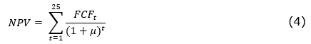
where μ is the risk-adjusted discount rate.
The main uncertainties of the project under analysis comprise the 3:2:1 crack spread, adjusted to the Brazilian market and the exchange rate. The definition of the stochastic processes to be used is based on the adjustment of the historical time series.
A refinery production is determined according to the derivatives demanded by the market. In the United States, gasoline demand is higher than diesel demand, so an American refinery is prepared to produce more gasoline than diesel, resulting in the 3:2:1 ratio, i.e. three barrels of oil producing 2 barrels of gasoline and 1 of diesel. In Brazil, the demand for diesel is higher than that of gasoline, so that Brazilian refining business should be adequate to produce more diesel than gasoline. Thus, the 3:2:1 crack spread can be adapted to the Brazilian reality, considering that three barrels of oil produce 2 barrels of diesel and 1 of gasoline.
Although 3:2:1 crack spread future contracts for different maturities are traded on the New York Mercantile Exchange (NYMEX), the embedded proportion corresponds to the North American market. To construct the crack spread adjusted to the Brazilian market, price data for oil, diesel and gasoline are extracted from the information of futures contracts traded in the North American market. The adjusted crack spread is than calculated as the price of a barrel of gasoline added to two times the price of a barrel of diesel and subtracting the price of three barrels of oil. Then, from the data of the adjusted crack spread, its deseasonalization is performed by decomposing into two factors (Heydari and Siddiqui, 2010):

where xt is the stochastic part and ft is a deterministic seasonal function.
The deterministic part can be described by a trigonometric function or using dummy variables, usually modeled from quarterly seasonality. The stochastic part can be modeled as an arithmetic mean reversion process known as the Ornstein-Uhlenbeck process, defined by the equation (6).

where x is the crack spread, η is the mean reversion speed, x̄ is the long-term equilibrium level, σx is the volatility, and dz is the Wiener increment.
To calculate the options values, assuming risk neutrality, in the case of the MRM process, the long-term equilibrium level is penalized by a risk premium (π) normalized by the mean reversion speed (Dias, 2015). Thus, in order to proceed with Monte Carlo simulation, the risk-neutral discretization of the MRM defined in equation (6) is given by:
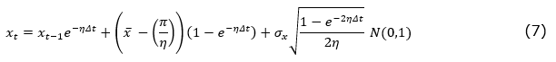
where the risk premium π = μ - r is the crack spread risk-adjusted discount rate minus the risk-free rate.
The uncertainty associated with the exchange rate is also important to evaluate a refinery in Brazil, given that oil and derivatives prices are formed in the international market. The exchange rate is commonly modeled as GBM, defined by equation (8).

where c is the exchange rate, α is the drift, σc is the corresponding volatility, and dz is the Wiener increment. The discretization under risk neutrality is given by equation (9).

where δc corresponds to the convenience yield of the exchange rate, which is the US dollar foreign risk-free rate.
To verify if the proposed processes can be used to describe the uncertainties, the Dickey-Fuller unit root test is performed, as well as the variance ratio test (Dias, 2015).
The option to postpone an investment may have an expiration date until when the decision should be made, or be perpetual, so that the decision can be made at any time. In addition, this option may be treated as function of one stochastic variable, given by the value of the project, or two stochastic variables, if the investment amount is modeled as a stochastic variable.
The value of the postponement option can be obtained based on the contingent claim method. Considering the value of the project as the underlying asset, the option value is obtained from the partial differential equation (PDE) of Black and Scholes (1973) and Merton (1973) given by equation (10).

where σV is the project volatility, V is the value of the project at t=0, δV is the cash flow distribution rate, and r is the risk-free rate.
These parameters are estimated from the Market Asset Disclaimer (MAD) method (Copeland and Antikarov, 2003). It is assumed that V has log-normal distribution, so it can be described as a GBM process, independently of the stochastic processes of the variables that influence its value. Considering that the MAD method simulates stochastic processes for all years of cash flow, which results in excessively high volatilities (Brandão et al., 2005a, 2005b; Smith, 2005), the stochastic processes are simulated only at time t = 1. For the other instants of time, the expected values of the stochastic processes are calculated from the simulated values at t = 1. Thus, it is possible to use the Monte Carlo simulation to simulate the stochastic components that affect the cash flows, obtaining the probability distribution of the project and extracting from this distribution the aggregate volatility of V.
If the decision to invest has no expiration date, the postponement option can be seen as perpetual. In this case, the EDP turns into an ordinary differential equation (ODE) that presents an analytical solution. The boundary conditions are given by equations (11) to (13).
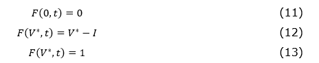
and the solution given by equations (14) (Dias, 2015):
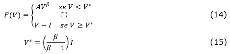
where V*, given by equation (15), is the threshold corresponding to the value from which the exercise of the option is optimal, β is the positive root of the characteristic equation of the ODE, and A is a constant determined by the boundary conditions.
If the option to wait to make the investment has an expiration date, it is characterized as an American option and can be exercised until the maturity date. In this case there is no analytical solution, and a numerical method should be used. Alternatively, Bjerksund and Stensland (1993) propose an analytical approximation method used in this paper.
A second approach to value the option to postpone is when the investment value (I) and the value of the project (V) are both considered stochastic. In this paper, given that the value of the investment is defined in domestic currency and the exchange rate is treated as a stochastic variable, the project is also evaluated from this perspective. Following McDonald and Siegel (1986), the option to postpone the investment is analyzed, in this case, based on the assumption that the two variables (V and I) follow correlated GBM processes. To reduce the dimensionality of the problem, the ratio v = V/I is used. The EDO, in this case, can be written according to equation (16).

where σ is the total volatility given by σ2 = σ2V - 2ρσVσI + σ2I, ρ is the correlation between V and I, and σI and δI are the volatility and the convenience yield of I, respectively, and the other parameters are the same presented in the EDP of Black and Scholes (1973) and Merton (1973). Similarly to equations (11) to (15), the boundary conditions are given by equations (17) and (18), the solution of the ODE by equation (19) and the trigger by equations (20).
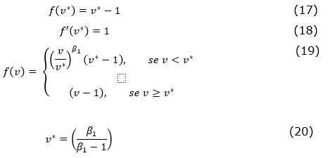
where β1 is the positive root of the characteristic equation of the ODE.
If the option value (F) is greater than the project NPV without flexibility, there is value on holding to make the investment. The investment decision must be taken from a critical value of the project called the threshold (V*). When the present value of the cash flows is greater than the critical value V*, the decision is to invest immediately. Otherwise, the best decision is to postpone the investment.
The option to temporarily shut down the refinery reflects the alternative to interrupt its operation for a certain period of time. It is assumed that the management can make this decision when the gross margin value, calculated as the crack spread, is lower than the variable costs.
The optimal operation mode is determined based on the values of the stochastic variables (crack spread and exchange rate) at each instant of time. As these variables change, the optimal mode can switch from operating to shutdown (and vice-versa). In this case, the cash flow should also include the cost of hibernation, relative to the conservation of the units while they are not operating.
The cash flow that encompasses the temporary shutdown option, here called as Optimal cash flow (Optimal CF), is defined as the maximum between the cash flow of the operating plant, which represents the cash flow without any flexibility, and the cash flow from hibernation, i.e. the costs incurred when the plant is not operating. Thus, at every instant of time, the optimal choice is made between operating or not:

where CFit is the cash flow at each time t for i = operating or hibernation.
The value of the temporary shutdown option is given by the difference between the expected present value of the optimal cash flow less the expected present value of the operating cash flow.
Finally, the interaction between the shutdown option and the option to postpone the investment should be assessed. The postponement option may lose value when incorporating a temporary shutdown option into the project, because the latter prevents large negative cash flows. Once including the temporary shutdown option, the MGB parameters of the project value are again estimated and the value of the postponement option is recalculated.
A database with daily data of 03/10/2005 until 02/28/2018 from NYMEX-traded prices provided by the Energy Information Administration (2018) was used to model the 3:2:1 crack spread. The following futures contracts with maturity of one month were considered: Cushing, OK Crude Oil, New York Harbor Regular Gasoline, New York Harbor Reformulated RBOB Regular Gasoline, and New York Harbor No. 2 Heating. The data was deflated for the same date using the Consumer Price Index (CPI), extracted from the Bureau of Labor Statistics (2018). The historical series is depicted in Figure 1:
Figure 1. Crack spread time series
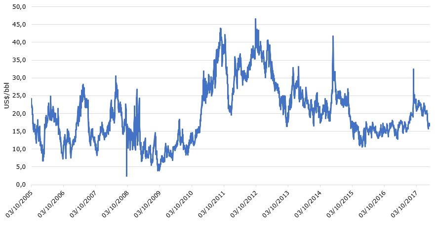
Source: Designed from Energy Information Administration (2018)
Using dummy variables to perform the deseasonalization of the quarterly series, the annual value of ft of approximately US$19/bbl was obtained in equation (5). For the stochastic part of the crack spread (xt), the Dickey-Fuller test was performed and the null hypothesis of the Brownian Arithmetic Movement (MAB) was rejected due to mean reversion behavior. Additionally, the variance ratio test was performed to confirm the existence of mean reversion, as shown in Figure 2:
Figure 2. Variance ratio test to crack spread
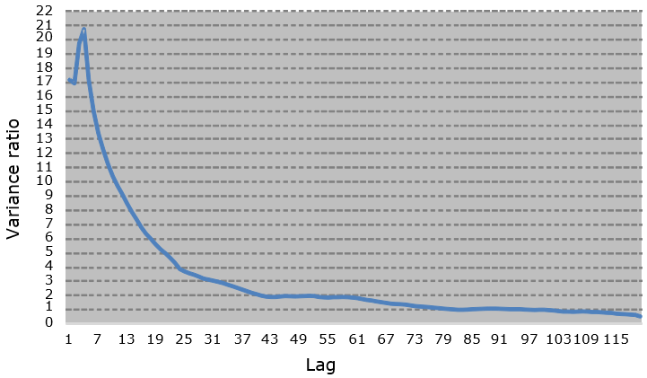
Source: The authors themselves
The estimated parameters of MRM process in equation (6) were σx = 18.38p.a. and η = 2.51. Due to the choice of the seasonal adjustment without intercept, the estimated long-term average x̄ was statistically zero.
The US Dollar / Brazilian Real exchange rate series used was modeled on daily data of 02/01/2002 to 02/28/2018, obtained from Institute for Applied Economic Research (Instituto de Pesquisa Econômica Aplicada - IPEA, 2018). The values were deflated based on the Consumer Price Index (CPI), obtained from the Bureau of Labor Statistics (2018), and the consumer price index (IPCA), from Brazilian Institute of Geography and Statistics (Instituto Brasileiro de Geografia e Estatística – IBGE, 2018). The results from Dickey-Fuller unit root test showed the MGB cannot be rejected, being appropriate to describe the stochastic process. In this case, the parameters found in equation (8) were σc=_15.74%p.a. and _α = -0.73%p.a.
Considering the cash flow described in US dollars, the risk-free rate of the US market was used in real terms (adopted estimate of 1%p.a.), in addition to the risk premium Brazil (adopted estimate of 3%p.a.), resulting in r = 4%p.a. Furthermore, the parameters of nominal capacity and utilization factor used in equation (1) and of income tax rate in equation (3) were, respectively, NC = 165,000 barrels per day, UF = 96% and τ = 34%.
Figure 3 shows the evolution of the accounts that make up the cash flow.
Figure 3. Expected cash flow
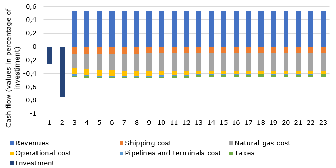
Source: The authors themselves
First, based only on the expected values of the traditional cash flow, i.e. disregarding the uncertainties associated with the crack spread and the exchange rate, and the existence of the proposed options, the present value of the project, V, obtained from the discounted cash flow, was US$ 2,575 million, resulting in a NPV of US$ 867 million for the case of incremental investment, and negative US$ 2,375 million for the case of the project not yet started.
To calculate the postponement option value, the parameters of the stochastic processes of the project value were estimated based on the MAD approach. Both cases with deterministic and stochastic investment were considered. The volatility and the convenience yield of V in equation (10) were estimated, respectively, as σV = 13.02% p.a. and δV = 4.24% p.a. The investment convenience yield in equation (16), based on the stochastic exchange rate, was estimated as δI = 1% p.a. The correlation between V and I was estimated as ρ=-0.67, based on correlation between the market prices of refining companies and the exchange rate.
From the simulation of the stochastic processes in the cash flow, the value of the project was calculated given the existence of the option to postpone the investment. Considering both the incremental investment and the total investment, Table 1 presents the values of the threshold V*, the option value F and the net premium of the option, given by the difference between F and the NPV, for different maturities.
Table 1. Postponement option results
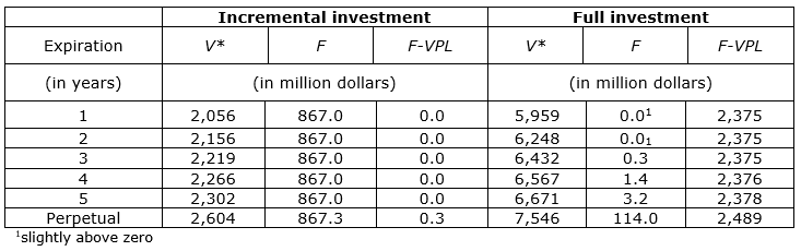
Source: The authors themselves
If the investment had not yet been started, i.e. if it had to be realized at its full value, the best decision would be to postpone the project regardless of the maturity of the option. For incremental investment, the recommendation is to invest immediately if the option expires in up to 5 years, but to defer it if the postponement option is perpetual.
Considering the incremental investment, the present value of the project is 1.5 times the value of the investment, which reduces the likelihood of loss in adverse scenarios. The cash flow distribution rate (δV= 4.24% p.a.), which represents the income obtained when making the investment and receiving the project cash flows, is higher than the risk-free rate (r= 4% p.a.), which represents the income that would have been received had the project not been made. Furthermore, the project volatility (σV= 13.02% p.a.) is not very high, which reduces the level of uncertainty associated with the investment cash flow. Therefore, these three factors explain why the postponement option has no value if the maturity is up to 5 years. In the case of perpetual option, despite those factors, the longer the time to expiration, the greater the possible change of the project value over time, leading to greater values of the option and the threshold.
In case of stochastic investment I, the ratio v is 1.5 in the scenario of incremental investment and 0.5 in the case of complete investment. The value found for v* in equation (20) is presented in Table 2, similar to the information presented in Table 1. Comparing v and v*, based on equation (19), the immediate investment is recommended only in the incremental case, when the expiration of the option is up to 2 years. The negative correlation between V and I increases the total volatility of the project, making it better to defer the project in some cases where the immediate investment was previously recommended when I was deterministic.
Table 2. Postponement option results for stochastic investment
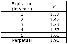
Source: The authors themselves
For the temporary shutdown option, the calculated expected optimum cash flow was US$ 2,782 million; thus, the presence of the option adds US$ 207 million of value to the NPV of the incremental project.
By incorporating the temporary shutdown option to the incremental project, the postponement option loses value. The option to defer had a positive value in the perpetual case; however, when interacting with the temporary shutdown option, the immediate investment turned to be the best decision, as it was for the cases where the option has an expiration date. For the full investment in a new refinery, although the postponement option has its value reduced, the decision is still to defer the project. In this case, the perpetual option was worth U$ 114 million, but by including the temporary shutdown option, the amount is reduced to U$ 14 million.
A sensitivity analysis is performed to verify how the parameters of volatility (σV) and cash flow distribution rate (δV) of the project could affect the analysis of the postponement in the case of incremental investment to complete the refinery.
When reducing σV to 8%p.a., the best decision is to invest immediately, and when increasing it to 35% p.a., it is recommended to postpone the investment decision, regardless of the expiration of the option. When the volatility is 20% p.a., if the expiration date is up to 3 years, the immediate investment is the best decision, but if the maturity of the option is higher, the investment should be postponed.
When increasing δV to 5% p.a., the best decision is to invest immediately, while the reduction to 2% p.a. indicates the postponement of project, regardless of the expiration date of the option. When δV is reduced to 3% p.a., if the option expires in 1 year, the best decision is to invest immediately, but the deferment of the investment is the recommended decision for all other expiration dates. These results indicate the importance of the prior definition of the expiration date for the deferment option, i.e. the deadline to make the decision.
For the case of stochastic I, a sensitivity analysis was performed based on the correlation ρ assuming values from -0.3 to -0.8. For ρ = -0.3, the deferral of the investment is recommended only if the option is perpetual, while for ρ = -0.8 the postponement is the best decision if the option expires in 3 years. If the project has not yet started, the investment decision involves an investment amount higher than the present value of the project. Thus, sensitivity analyzes were made for I = 3.55, 3.0, and 2.5 million dollars. Although in the latter case the traditional analysis recommends the realization of the investment (because NPV>0), when evaluating the option to postpone, the best decision is still the deferral of the project in those three scenarios.
The temporary shutdown is affected by the cost of hibernation of the units. Three scenarios were analyzed, with hibernation cost of US$ 5, 11, and 44 million. The value of the temporary shutdown option for each scenario was, respectively, US$ 214, 213, and 194 million dollars. A change in the cost of hibernation generates modest gains in the result of the optimal cash flow and, consequently, in the option value, which explains the small variation of these observed results. This is because, although in a few years the cash flow of the operation is negative, there are few scenarios in which the present value of the cash flows of the whole project is negative, which can be seen in Figure 4.
Figure 4. Distribution of the present value of operation cash flows
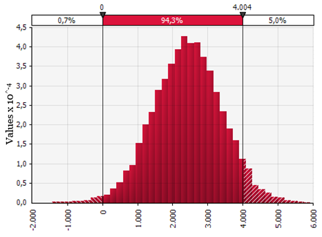
Source: The authors themselves
To analyze an oil refinery in Brazil, this work modeled the main uncertainties associated with the investment: the crack spread and the exchange rate. It was proposed an adaptation of the 3:2:1 crack spread for the Brazilian market, the main uncertainty of the cash flow of a refinery, to reflect the reality of national refining. The time series present a mean-reversion behavior and, when considering the seasonality, it is possible to model the stochastic process as an arithmetic move.
Given the complexity of oil refinery projects and the high amount of investment involved, the correct valuation of the embedded managerial flexibilities based on the real options approach is an important issue. Considering that there are refinery projects in Brazil that were interrupted before completion and that the country is a derivative importer, the analysis of the postponement option can be considered especially relevant. Also, Brazil is an oil-producing country; thus, the temporary shutdown option corresponds to the possibility of comparing what is worth: producing derivatives or increasing the volume of oil to export. In addition to the value added by each of these options in the project, the interaction between them was also considered in this paper.
In the proposed project, the real option approach determined the postponement of investment in situations where the traditional analysis of discounted cash flow recommended the immediate investment.
For the remaining investment to complete 15% of the refinery the traditional analysis presented a positive NPV; however, the real option valuation pointed in a different direction depending on the expiration date of the option. The postponement of the project for the remaining investment was the best decision if the option to wait to make the investment is considered perpetual, since the value of the option was small in most cases. However, in case of expiration within one year, most of the cases led to the immediate investment recommendation. These conclusions reflect the results found for most of the scenarios studied, but when performing sensitivity analysis there are some cases that result in different decision, reducing robustness of the results. For the other expiration dates over one year, the decision presented large variations in the scenarios analyzed.
For the case where the full investment is considered for a new refinery, the best decision is always to postpone the investment.
The temporary shutdown option was also evaluated considering the change of mode between operating and not operating the refinery. In all cases proposed, this option added value to the refinery's result. In addition, the temporary shutdown option reduced the value of the postponement option; thus, the immediate investment of the incremental amount for the refinery completion is recommended regardless of its expiration date.
Future work can be suggested. First, the modeling of crack spread data of the Brazilian market, considering the domestic prices of the derivatives and reflecting data closer to the reality of the country, may enrich studies in the refinery industry. Second, stochastic crack spread modeling can also be improved by using two- or three-factor mean reversion models, or including jumps in the model, to better reflect the long-run crack spread, since the mean reversion model does not capture long-term trends for the equilibrium price level. In addition, natural gas price could also be incorporated into the model by modeling a third stochastic variable, since, disregarding oil, it is a significant cost to the refinery. Finally, switch options especially related to the inputs used can also be incorporated from the crack spread modeling approach.
Aiube, F.A.L. (2013), Modelos Quantitativos em finanças com enfoque em commodities, Bookman, Porto Alegre.
Azevedo, T.C., Aiube, F.L., Samanez, C.P., Bisso, C.S. and Costa, L.A. (2015), “The behavior of West Texas Intermediate crude-oil and refined products prices volatility before and after the 2008 financial crisis: an approach through analysis of futures contracts”, Ingeniare. Revista Chilena de Ingeniería, Vol. 23, No. 3, pp. 395–405.
Bjerksund, P. and Stensland, G. (1993), “Closed-form approximation of American options”, Scandinavian Journal of Management, Vol. 9, pp. S87–S99.
Black, F. and Scholes, M. (1973), “The Pricing of Options and Corporate Liabilities”, Journal of Political Economy, The University of Chicago Press, Vol. 81, No. 3, pp. 637–654.
Brandão, L.E.T., Dyer, J.S. and Hahn, W.J. (2005a), “Using Binomial Decision Trees to Solve Real-Option Valuation Problems”, Decision Analysis, INFORMS, Vol. 2, No. 2, pp. 69–88.
Brandão, L.E.T., Dyer, J.S. and Hahn, W.J. (2005b), “Response to Comments on Brandão et al. (2005)”, Decision Analysis, INFORMS, Vol. 2 No. 2, pp. 103–109.
Bureau of Labor Statistics. (2018), “Bureau of Labor Statistics”, Historical Consumer Price Index for All Urban Consumers, available at: https://www.bls.gov/cpi/tables/supplemental-files/historical-cpi-u-201802.pdf (accessed 20 February 2018).
Castro Lopes, C. et al. (2020), “Valuation of a crude oil refinery in Brazil under a real options approach”, in Leiras A. et al. (Eds.), Operations Management for Social Good, 2018 POMS International Conference in Rio, Springer Proceedings in Business and Economics Series, Springer International Publishing. In press.
Clews, R. (2016), Project Finance for the International Petroleum Industry, Academic Press. Copeland, T.E. and Antikarov, V. (2003), Real Options: A Practitioner’s Guide, Texere.
Costa, L.A. and Samanez, C.P. (2009), “Análise e avaliação de flexibilidades input output em projetos de plantas na industria do petróleo: uma aplicação da teoria das opções reais e da simulação estocástica”, GEPROS - Gestão Da Produção, Operações e Sistemas, Vol. 4, No. 2, pp. 63–78.
Dempster, M.A.H., Medova, E. and Tang, K. (2008), “Long term spread option valuation and hedging”, Journal of Banking & Finance, Vol. 32, No. 12, pp. 2530–2540.
Dias, M.A.G. (2014), Análise de investimentos com opções reais - Teoria e prática com aplicações em petróleo e em outros setores, Vol. 1: Conceitos básicos e opções reais em tempo discreto, Interciência, Rio de Janeiro.
Dias, M.A.G. (2015), Análise de investimentos com opções reais - Teoria e prática com aplicações em petróleo e em outros setores, Vol. 2: Processos estocásticos e opções reais em tempo contínuo, Interciência, Rio de Janeiro.
Dixit, A.K. and Pindyck, R.S. (1994), Investment under Uncertainty, Princeton University Press, Princeton.
Dunne, T. and Mu, X. (2010), “Investment Spkies and Uncertainty in the Petroleum Refining Industry”, The Journal of Industrial Economics, Wiley, Vol. 58. No. 1, pp. 190–213. Energy Information Administration. (2018), “NYMEX Futures Prices”, available at: https://www.eia.gov/dnav/pet/pet_pri_fut_s1_d.htm (accessed 20 March 2018).
Fonseca, D.A.D. (2008), Avaliação de projetos de investimento com opções reais: cálculo de valor de opção de espera de uma unidade separadora de propeno, Master Dissertation, Escola de Pós-Graduação em Economia (EPGE), Fundação Getúlio Vargas (FGV), Rio de Janeiro, available at: https://bibliotecadigital.fgv.br/dspace/handle/10438/1752 (accessed 20 March 2018).
Heydari, S. and Siddiqui, A. (2010), “Valuing a gas-fired power plant: A comparison of ordinary linear models, regime-switching approaches, and models with stochastic volatility”, Energy Economics, Vol. 32, No. 3, pp. 709–725.
Imai, J. and Nakajima, M. (2000), “A real option analysis of an oil refinery project”, Financial Practice and Education, Vol. 10, pp. 78–91. Instituto Brasileiro de Geografia e Estatística - IBGE. (2018), “Tabelas Históricas IPCA, INPC”, available at: https://ww2.ibge.gov.br/home/estatistica/indicadores/precos/inpc_ipca/defaultseriesHist.shtm (accessed 4 June 2018).
Instituto de Pesquisa Econômica Aplicada - IPEA. (2018), “IPEA Data”, available at: http://ipeadata.gov.br/Default.aspx (accessed 4 June 2018). Kemna, A.G.Z. (1993), “Case Studies on Real Options”, Financial Management, [Financial Management Association International, Wiley], Vol. 22, No. 3, pp. 259–270.
Kulatilaka, N. and Trigeorgis, L. (1994), “The General Flexibility to Switch: Real Options Revisited”, International Journal Of Finance, Vol. 6, No. 2, available at:https://doi.org/https://ssrn.com/abstract=5567.
Leiras, A., Hamacher, S. and Scavarda, L.F. (2008), “An Integrated Supply Chain Perspective Evaluation for Biodiesel Production in Brazil”, Brazilian Journal of Operations & Production Management, Vol. 5, No. 2, pp. 29–47.
Li, Y., Tseng, C.-L. and Hu, G. (2015), “Is now a good time for Iowa to invest in cellulosic biofuels? A real options approach considering construction lead times”, International Journal of Production Economics, Vol. 167, pp. 97–107.
McDonald, R. and Siegel, D. (1986), “The Value of Waiting to Invest”, The Quarterly Journal of Economics, Vol. 101, No. 4, pp. 707–727.
Merton, R.C. (1973), “Theory of Rational Option Pricing”, The Bell Journal of Economics and Management Science, Vol. 4, No. 1, pp. 141–183.
Minardi, A.M.A.F. (2000), “Teoria de opções aplicada a projetos de investimento”, Revista de Administração de Empresas, Vol. 40, pp. 74–79.
O’Driscoll, P.J. (2016), A Study in the Financial Valuation of a Topping Oil Refinery, Doctorate Thesis, Birkbeck College, University of London, London, available at: http://bbktheses.da.ulcc.ac.uk/232/.
Oliveira, C.A. de. (2014), “Investment and exchange rate uncertainty under different regimes”, Estudos Econômicos (São Paulo), Vol. 44, pp. 553–577.
Pindyck, R.S. (1999), “The Long-Run Evolution of Energy Prices”, The Energy Journal, International Association for Energy Economics, Vol. 20, No. 2, pp. 1–27.
Pindyck, R.S. (2001), “The Dynamics of Commodity Spot and Futures Markets: A Primer”, The Energy Journal, International Association for Energy Economics, Vol. 22 No. 3, pp. 1–29.
Población, J. and Serna, G. (2016), “Is the refining margin stationary?”, International Review of Economics & Finance, Vol. 44, pp. 169–186.
Sharma, P., Romagnoli, J.A. and Vlosky, R. (2013), “Options analysis for long-term capacity design and operation of a lignocellulosic biomass refinery”, Computers & Chemical Engineering, Vol. 58, pp. 178–202.
Smith, J.E. (2005), “Alternative Approaches for Solving Real-Options Problems”, Decision Analysis, INFORMS, Vol. 2, No. 2, pp. 89–102.
Teles, V.K. (2005), “Choques cambiais, política monetária e equilíbrio externo da economia brasileira em um ambiente de hysteresis”, Economia Aplicada, Vol. 9, No. 3, pp. 415-426.
Trigeorgis, L. (1993), “The Nature of Option Interactions and the Valuation of Investments with Multiple Real Options”, The Journal of Financial and Quantitative Analysis, Cambridge University Press, Vol. 28, No. 1, pp. 1–20.
Vianello, J.M. and Teixeira, J.P. (2012), “Valoração de Opções Reais Híbridas em Projetos Modularizados: Uma Metodologia Robusta para Investimentos Governamentais e Privados”, Revista Pensamento Contemporâneo Em Administração, Vol. 6, No. 2, pp. 103–129.
Vianello, J.M., Costa, L. and Teixeira, J.P. (2014), “Dynamic modeling of uncertainty in the planned values of investments in petrochemical and refining projects”, Energy Economics, Vol. 45, pp. 10–18.
Yabiko, R.F. and Bone, R.B. (2016), “The Pressures of the Brazilian Pre-Salt Production on the National Refining Sector”, Brazilian Journal of Operations & Production Management, Vol. 13, No. 3, pp. 344–350.
Yi, C. (1997), Real and Contractual Hedging in the Refining Industry, Doctorate Thesis.
Received: 28 Feb 2019
Approved: 21 Jun 2019
DOI: 10.14488/BJOPM.2019.v16.n3.a2
How to cite: Lopes, C. C.; Blank, F. F.; Thomé, A. M. T. et al. (2019), “Investment decisions in an oil refinery in Brazil under a real option approach”, Brazilian Journal of Operations & Production Management, Vol. 16, No. 3, pp. 375-386, available from: https://bjopm.emnuvens.com.br/bjopm/article/view/789 (access year month day).