
São Paulo State University (Unesp), Campus of Itapeva, São Paulo, Brazil.
São Paulo State University (Unesp), Campus of Itapeva, São Paulo, Brazil.
São Paulo State University (Unesp), Campus of Itapeva, São Paulo, Brazil.
Goal: In this paper, a binomial model is proposed to evaluate the option of deferring an investment and expanding the operational scale of a forest-based company that will perform the de-duplication of Pinus sp. and will market packaging for storage and transportation of vegetables.
Design/Methodology/Approach: The proposed model measured the options of deferring an investment and expanding the operational scale of the forest-based company. In this perspective, the model of evaluation used was the binomial model in discrete time using the Real Options.
Results: It was observed that the inclusion of management flexibilities in the decision making process has added value to the investment project; therefore, the project of investments in real assets proved to be economically feasible.
Limitations of the investigation: The studies that address the corporate finance framework based on real data are a restrictive factor, due to the lack of collaboration of companies, that is, the availability of information that is usually classified.
Practical implications: The study was based on the real data of a company; therefore, it can be adopted as a stimulus to the Real Options approach to the decision making of entrepreneurs or researchers.
Originality/value: The focus of the study was to contemplate the managerial flexibilities of an industry of the secondary sector of the Brazilian economy, which performs the unfolding of wood, demonstrating the innovation of the technique approach used in this market segment.
Keywords: Economic evaluation; uncertainties; binomial model; volatility.
Successful economic and market development requires the application of traditional methods in business and the application of new modern methods adapted to the contemporary market needs, requirements and conditions. The application of this methodology consists of evaluating the suitability, efficiency and feasibility of the project, in order to make a final conclusion on whether a proposed investment project is profitable. These methods are mostly based on the comparison of the necessary expenditures and the derived revenues (Dikareva and Voytolovskiy, 2016; Rajnoha et al., 2014; Sujová and Marcineková, 2015).
The most widely used methodology is the discounted cash flow (DCF) analysis, which discounts the balances between costs and revenues within the estimated duration of the investment. The prominent reasons for the usage of DCF techniques by the vast majority of companies are their consideration of time value of money as well as the ability of assessing the wealth of an organization in a period of time. Hence, the cash flow can recognize whether the investment project has successfully sustained over this time interval or not, showing the profits and loss during the project life (Batra and Verma, 2017; Iyer and Kumar, 2016; Sdino et al., 2016; Oliveira and Zotes, 2018).
However, the DCF analysis needs accuracy and it assumes that the scenario and the project life are fixed. According to this approach, the manager will not be able to react to environmental changes and may be in danger of bankruptcy. Therefore this method fails to capture the uncertainties, not proposing the accurate consideration of variations in the environment. It was Myers (1984) who first acknowledged these limitations with standard DCF approaches when it comes to valuing investments with significant options (Kokkaew and Sampim, 2014; Pivorienė, 2015; Ugwuegbu, 2013; Braga et al., 2018).
To overcome the lack of flexibility integration of traditional capital budgeting methods, one can apply the analysis of real options. The technique of applying real options to the evaluation of projects includes factors that the classical methodology – in some cases – has left aside, such as flexibility, uncertainty and volatility. Through the inclusion of these components, one can reach a much more dynamic analysis, because the real options theory views investments as rights but not obligations, conducting the investment's values to be maximized (Čirjevskis and Tatevosjans, 2015; Hammann et al., 2017; Tanaka and Montero, 2016).
Thus, a real option is the right, but not the obligation, to undertake an action, at a predetermined cost, called the exercise price, for a pre-established period: the life of the option. Real options can be divided into investment timing option, operational flexibility option, abandonment option, and growth option. These options can be taken during the execution of the project with the aim of maximizing results or eliminating losses (Copeland and Antikarov, 2002; Lupo and Reiner, 2017; Santos et al., 2015).
From this perspective, a stochastic process becomes appropriate to address a problem that requires good uncertainty modeling as it helps increase confidence in the results. One of the most important basic notions of stochastic processes is Brownian Motion (also called a Weiner process) or Geometric Brownian Motion (GBM). In economic applications the GBM have extensively been used, because it is a common specification to model asset values (Bastian-Pinto, 2015; Carlander et al., 2016; Chávez-Bedoya, 2016; Sampim et al., 2017; Schachter et al., 2016).
For this modeling, it is possible to use the binomial model. The most used binomial valuation model corresponds to the proposal developed by Cox et al. (1979), which is usually adopted for the real options analysis and is based on the creation of recombinant binomial trees that determine the paths that the price of the asset evaluated follows until the time of expiration. The main idea of the binomial model is to replace a continuous distribution of share prices by a simple two-point discrete distribution, keeping the technical framework on a very low level (Bock and Korn, 2016; Cuervo and Botero, 2014; Perufo et al., 2017; Yuen et al., 2013).
The Binomial model proposal is attractive from the academic point of view because it maintains a precise economic view of the traditional models of options pricing and can be easily understood. Thus, the use of more dynamic valuation methodologies, which can add value to investment projects, are necessary. Therefore, the aim was to develop a binomial model to evaluate the economic viability of a forest-based company’s investment project in real assets, including managerial flexibilities for postponing the investment and expanding the operational scale.
The study was developed from the technical-economic coefficient of a forest-based company to be installed in the Southwest region of the State of São Paulo, whose activity will consist of log breakdown of Pinus sp. with diameters from 14 cm to 30 cm and a maximum length of 2.5 m, with the capacity to saw 950 cubic meters of wood per month. From lumber the packaging for storing and transporting vegetables will be produced.
The economic mission of the company will be the unfolding wood, according to the National Classification of Economic Activities (CNAE), registered under the class number 1610-2. In addition, the Simplified National Tax (Simples Nacional) with annual billing of one million US dollars was used to calculate the company's operating performance for the processing of the manufacturing industry's tax activities. Hence, a single amount will be 19.00%, which will be distributed in taxes: 13.50% Corporate Income Tax; 10.00% Social Contribution on Net Income; 28.72% Contribution to Social Security Financing; 6,13% Social Integration Program; 42.10% Employer Social Security Contribution (Employer Pension Contribution - EPC).
Monetary values were expressed in US dollars (USD), using the exchange rate of R$ 3.6913 according to information provided by the Central Bank of Brazil (Banco Central do Brasil, 2018) on 06/11/2018. The Weighted Average Capital Cost (WACC) was considered, as it was adjusted to the risk-free rate as proposed by Copeland et Antikarov (2001), according to Equation 1. In this way, the discount rate of the investment project was determined as the minimum rate of return (MRR), i.e. the rate of return required by investors to bring cash flows to the present date.
where:
Ke is the cost of equity;
Kd is the cost of debt;
Kp is the market value of equity;
Kt is the market value of debt;
Tc is the corporate tax rate.
Thus, a risk-adjusted discount rate, obtained through the Capital Asset Pricing Model (CAPM), was estimated, according to Equation 2.

where:
K is the risk-adjusted discount rate;
Rf is the risk free rate (10 years T-Bills rates);
β is the systematic risk;
RM is the expected market return (S&P Global Timber & Forestry Index);
αBR is the country risk premium.
Considering the parameters of Equation 2, the 2.84% risk-free interest rate issued by the United States Department of the Treasury was used because it was reasonably integrated with the world capital market. Furthermore, the beta value of 1.2 was considered as a measure of the systemic risk of the forest products, and the expected market return in the S & P Global Timber & Forestry Index was 3.42%. The country risk premium of 2.61% was weighted, in accordance with the arithmetic mean of the last ten years of the Emerging Markets Bonds Index – EMBI + Br.
The discounted cash flow (DCF) which determines the value of the company, was considered as conventional, that is, it presents a single capital expenditure (CAPEX) followed by several operating cash inflows, taking into consideration a horizon projection of 10 years, which allows us to predict the behavior of revenues and operational expenditure (OPEX) in a plausible way. However, for the cash flows not contemplated in this horizon, the perpetuity was assumed to have a zero growth rate; therefore, it was considered that the company has an infinite financial life.
Consequently, it was possible to calculate the net present value without the managerial flexibilities, that is, the traditional net present value according to Equation 3.

where:
T is the duration of the project;
t is the time period in which costs and revenues occur;
i is the minimum rate of return;
CFt is the cash flow for t periods;
I is the value of the initial investment.
The standard deviation of the returns, that is, the project volatility, was calculated using the methodology proposed by Brandão et al. (2012), which evaluates the volatility in the first year, conditioned to the expectations of the present values in the other years of the project, assuming that the variations in the cash flows are independent, and that the volatility is constant throughout the horizon projected. Knowing that the uncertainties affect the relevant project variables and their impact on returns can be determined by means of the stochastic processes’ simulation, it was assumed that the fixed asset price volatility follows a GBM described in Equation 4, as predicted by Dixit et Pindick (1994).

where:
P is the price of the asset at time t;
μ is the rate of growth of P (drift);
σ is volatility;
dz is the increment of a Wiener process;
Thus, the volatility, i.e. the percentage standard deviation of the project return, was calculated (Equation 5), as Copeland et Antikarov (2001) recommend.

where:
z is the percentage change in the value of the project;
ln is the neperian logarithm;
PV0 is the present value at time t = 0;
PV1 is the present value at time t = 1;
CF1 is the free cash flow at time t = 1.
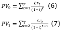
To calculate the present value of the project at instants t = 0 and t = 1, we used Equations 6 and 7, respectively.
Moreover, it was assumed that the main uncertainty which affected the project’s value was the revenues obtained with the commercialization of the packages, that followed a lognormal distribution with mean α and standard deviation σ, ensuring that only positive values were obtained, considering the assumption of the GBM. The simulation was performed using the software @Risk Copyright © 2017 Palisade Corporation (Palisade, 2017), with the generation of 100,000 pseudorandom numbers.
The project has managerial flexibilities to postpone the investment, which is equivalent to a call option of american stocks and to expand the operational scale, also formally equivalent to a call option. In this way, investment in fixed assets could be exercised in the second year, while the option to expand by 30% the operational scale could be carried out in the tenth year of the project if the company made the investment.
In order to evaluate the real options, the binomial model of Cox et al. (1979) was applied. This model predicts the behavior of the price of the underlying asset, that is, the physical project that is under evaluation, and can assume two values in the future, according to the up and down multiplicative factors.
The values of the multiplicative factors, represented by up (u) and down (d) factors are based on the volatility of the underlying asset and the expiration time and were obtained by means of Equation 8 and 9, respectively.

where:
∆t is the time variation that corresponds to the size of the step between the nodes of the binomial tree;
e is the constant 2.71828...;

with u > d.
To determine the probability of occurrence of these movements, the risk-neutral probability (p) was used. Thus, the investment project has the probability p of increasing its value, or the probability q = 1 - p, of decreasing this value, calculated according to Copeland et Antikarov (2001), described in Equation 10.

Thus, with the multiplicative factors and the calculated probabilities, it was possible to construct the binomial tree in discrete time using the dynamic programming language software DPL 9 (Syncopation, 2018).
In view of this, once the present value modeling of the project has been defined and structured, the inclusion of managerial flexibilities was made by inserting the decision instant in which the project value function is maximized. The present value of the project in the binomial tree was calculated in each node of the tree, considering whether or not the company manager should perform the option to achieve the optimal result.
The real option value (ROV) is given by the difference between the present value of the project with the included flexibilities and the traditional present value, derived from discounted cash flow analysis. Consequently, the net present value expanded (NPVEXP) was obtained, using the traditional net present value and the real option value, by means of Equation 11, in agreement with Trigeorgis (1995).

Capital expenditures (CAPEX) were accounted in the initial investment year in the amount of USD 862,079.93, and, when weighting OPEX, depreciation and the taxes calculated by the traditional investment analysis method, allowed determining that the present investment project value was USD 1,756,218.11.
However, when applying the simulation by the Monte Carlo method, it was found that this resulted in the average value of USD 1,757,801.67 and a standard deviation of USD 782,512.53, confirming the presence of volatility (Figure 1). Thus, the Monte Carlo simulation proved to be an effective tool for advising the decision maker and helping in corporate risk management (Laudares et al., 2019).
The project’s volatility is the uncertainty over expected project returns from period to period (Godinho, 2006). Therefore, particularly the price of the asset object will depend on this volatility, that is, the level of uncertainty of the project to be weighed in the model.
Figure 1. Distribution of probability of the present value
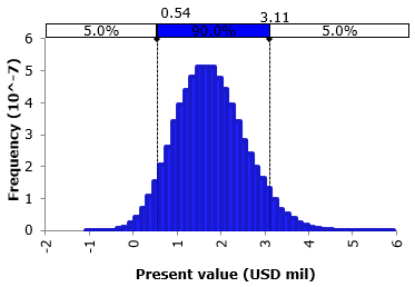
Source: The authors themselves.
It should also be noted that the probabilistic distribution resulted in an asymmetry of 0.3019 and kurtosis of 3.1295. These values indicate the lognormality of the data, thereby, it is assumed that the returns of the project are normally distributed, so that the value of the project has lognormal distribution and can be approximated through a binomial mesh (Brandão and Dyer, 2009).
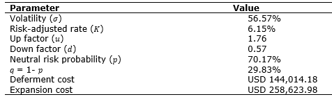
After identifying all relevant options, it is possible to employ the real options methodology by constructing a binomial model (Hartmann and Hassan, 2006). One of the most important factors for this analysis is the volatility, by explaining the behavior of the asset price object, so the investment project's volatility under analysis was 56.57%. In addition, the other parameters intrinsic to the application of the Real Options Theory, such as multiplicative factors (up and down), risk-adjusted rate, objective probabilities, and monetary values demanded by managerial flexibilities, are presented in Table 1.
Table 1. Parameters that affect real option’s value.
Moreover, as the project can be postponed in the second year of its useful life and the operational scale can be expanded by 30% in the last year, a decision node that models the managerial flexibility that exists in the project is inserted, as shown in Figure 2.
Figure 2. Binomial model of the investment project
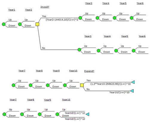
Source: The authors themselves.
According to Copeland et al. (2002), when decision intersections are added to an event tree, it becomes a decision tree. Hence, with the inclusion of management flexibilities, the present value of the updated investment project was obtained through the decision tree. It was observed that the decision tree includes bold lines that highlight the optimal decision, being a more intuitive tool for the decision maker.
Decision trees are tools that can be used for making financial decisions, providing an effective structure in which alternative decisions and the implications of taking those decisions can be laid down and evaluated; besides that, they also help to form an accurate, balanced picture of the risks and rewards that can result from a particular choice (Carlsson and Fullér, 2003).
With the valuation of the option, the project’s present value is presented in the node referring to Year 1 (Figure 3). In this sense, the present value of the project obtained from the real options was USD 3,823,634.20, with a standard deviation of USD 88,163.81.1, the minimum amount of USD 378,346.80, and the maximum value of USD 364,414,971.70.
The NPV with the flexibilities of deferring and expansion was higher when compared to the traditional NPV; thus, it was possible to quantify the right to exercise the real options, suggesting that the investor could exercise them because it allowed maximizing the value of the opportunity of investments. In this way, according to Luehrman (1988), the corporate investment opportunity is a call option because the corporation has the right, but not the obligation to acquire something.
Figure 3. Decision tree up to the third year of project life
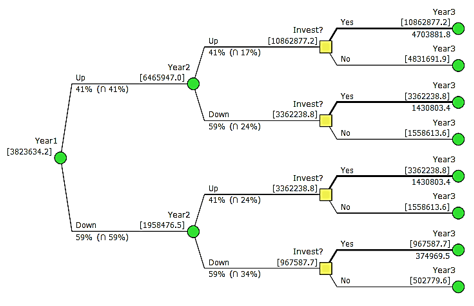
Source: The authors themselves.
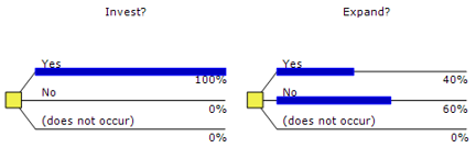
The decision tree demonstrates the scenarios for decision making, that is, an optimal decision to be made by the investment project manager. In this sense, it is observed in Figure 4 that all paths demonstrate the feasibility of making an investment, since in 100% of the investment opportunities it is possible. Nonetheless, only 40% of the opportunities are interesting for the decision maker to expand the operational scale, indicating that it is subject to the risk of witnessing an environment that is not conducive to the intensification of activities. Furthermore, it can be seen that the managerial flexibilities increased the value of the project, considering that the value generated by the real options was USD 2,067,416.09, and thus, the USD 2,921,554.27 were obtained. However, it is important to note that the increase in economic parameters may have been influenced by the volatility of the investment project.
Figure 4. Optimal investment policy
Source: The authors themselves.
According to Miller et Waller (2003), the real options and the expected present value of the project are positively influenced by the volatility. In view of this, the greater the volatility of the investment project, the higher the expected value and the lower the likelihood of executing the expansion option. Therefore, the level of uncertainty has been shown to exert a positive effect on the price of the underlying asset.
Figure 5. Sensitivity analysis of the project's expected present value
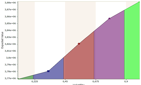
Source: The authors themselves.
The traditional cash flow methodology is a widely used investment valuation technique. However, this technique fails to capture the managerial flexibilities present in investment projects inserted in dynamic environments. This paper presents a model for the evaluation of investments under the real options perspective, considering the options for postponing and expanding the productive scale of a forest-based industry in the second and tenth year of the project life, respectively.
The binomial model is considered a simple and straightforward way of evaluating real options, in addition to demonstrating the optimal scenario for decision making. Thus, it was observed that the postponement option would not be used, because in all the paths generated by the decision tree, the option to invest proved viable. Regarding the expansion option, it is suggested that in 60% of the opportunities the expansion should not be performed.
The volatility present in the investment project corroborated the presence of uncertainty to be weighed in the evaluation of investments, and it is one of the fundamental parameters as input of the binomial model. By means of the sensitivity analysis it was concluded that the volatility has a direct relationship with the expected present value, i.e. the higher the volatility value, the greater the present value. However, for the analyzed condition, there will be a decrease in the probability of expanding the operational scale.
There had been an increase of 231% in investment project when compared to the estimated calculation based on the traditional investment analysis methodology.
We thank FAPESP for a scholarship granted to the first author - grant #2017/20323-0, São Paulo Research Foundation (FAPESP).
Banco Central do Brasil (2018), Conversão de Moedas, available from: http://www4.bcb.gov.br/pec/conversao/conversao.asp (acess 11 Jun. 2018).
Bastian-Pinto, C. L. (2015), “Modeling generic mean reversion processes with a symmetrical binomial lattice - applications to real options”, Procedia Computer Science, Vol. 55, pp. 764-773.
Batra, R.; Verma, S. (2017), “Capital budgeting practices in Indian companies”, IIMB Management Review, Vol. 29, pp. 29-44.
Bock, A.; Korn, R. (2016), “Improving convergence of binomial schemes and the edgeworth expansion”, Risks, Vol. 4, No. 4, pp.15-22.
Braga, F. J. A. et al. (2018), “Analysis of individual micro-entrepreneur vision from the perspective of financial management”, Brazilian Journal of Operations & Production Management, Vol. 15, No. 2, pp.182-192.
Brandão, L. E. T. et al. (2012), “Volatility estimation for stochastic project value models”, European Journal of Operational Research, Vol. 220, No. 3, pp. 642-648.
Brandão, L. E. T.; Dyer, J. (2009), “Projetos de opções reais com incertezas correlacionadas”, Revista Base, Vol. 6, No. 1, pp. 19-26.
Carlander, L. et al. (2016), “Integration of cost-risk assessment of denial of service within an intelligent maintenance system”, Procedia CIRP, Vol. 47, pp. 66-71.
Carlsson, C.; Fullér, R. (2003), “A fuzzy approach to real option valuation”, Fuzzy sets and systems, Vol. 139, No. 2, pp. 297-312.
Chávez–Bedoya, L. (2016), “Determining equivalent charges on flow and balance in individual account pension systems”, Finance and Administrative Science, Vol. 21, No. 40, pp. 2-7.
Čirjevskis, A.; Tatevosjans, E. (2015), “Empirical testing of real option in the real estate market”, Procedia Economics and Finance, Vol. 24, pp. 50-59.
Copeland, T. E. et al. (2002), Avaliação de empresas – Valuation: calculando e gerenciando o valor das empresas, Pearson Makron Books, São Paulo.
Copeland, T. E.; Antikarov, V. (2002), Opções Reais: Um novo paradigma para reinventar a avaliação de investimentos, Campus, Rio de Janeiro.
Copeland, T.; Antikarov, V. (2001), Real options, Texere, New York.
Cox, J. et al. (1979), “Option pricing: A simplified approach”, Journal of Financial Economics, Vol. 7, No. 3, pp. 229–263.
Cuervo, F. I.; Botero, S. B. (2014), “Aplicación de las opciones reales en la toma de decisiones en los mercados de electricidad”, Estudios Gerenciales, Vol. 30, No. 133, pp. 397-407.
Dikareva, V.; Voytolovskiy, N. (2016), “The efficiency and financial feasibility of the underground infrastructure construction assessment methods”, Procedia Engineering, Vol. 165, pp. 119-1202.
Dixit, A.; Pindyck, R. (1994), Investment under uncertainty, Princeton Press, Princeton.
Godinho, P. (2006), “Monte Carlo estimation of project volatility for real options analysis”, Journal of Applied Finance, Vol. 16, No. 1, pp. 15-30.
Hammann, E. et al. (2017), “Economic feasibility of a compressed air energy storage system under market uncertainty: a real options approach”, Energy Procedia, Vol. 105, pp. 3798-3805.
Hartmann, M.; Hassan, A. (2006), “Application of real options analysis for pharmaceutical R&D project valuation—Empirical results from a survey”, Research Policy, Vol. 35, No. 3, pp. 343-354.
Iyer, K. C.; Kumar, R. (2016), “Impact of delay and escalation on cash flow and profitability in a real estate project”, Procedia Engineering, Vol. 145, pp. 388-395.
Kokkaew, N.; Sampim,T. (2014), “Improving economic assessments of clean development mechanism projects using real options”, Energy Procedia, Vol. 52, pp. 449-458.
Laudares, A. C. et al. (2019), “When does it end? Monte Carlo simulation applied to risk management in defense logistics’ procurement processes”, Brazilian Journal of Operations & Production Management, Vol. 16, No. 1, pp.149-156.
Luehrman, T. A. (1988), “Investment opportunities as real options: getting started on the numbers”, Harvard Business Review, pp. 51-57.
Lupo, S.; Reiner, D. M. (2017), “How does changing the penetration of renewables and flexibility measures affect the economics of CCS penetration?”, Energy Procedia, Vol. 114, pp. 7596-7600.
Miller, K. D.; Waller, H. G. (2003), “Scenarios, real options and integrated risk management”, Long Range Planning, Vol. 36, No. 1, pp. 93-107.
Myers, S. C. (1984), “The capital structure puzzle”, Journal of Finance, Vol. 39, pp. 575–592.
Oliveira, F. B.; Zotes, L. P. (2018). “Valuation methodologies for business startups: a bibliographical study and survey”, Brazilian Journal of Operations & Production Management, Vol. 15, No. 1, pp. 96-111.
Palisade Corporation. (2017). Versão 7.5.2, @Risk, Newfield, Palisade Corporation.
Perufo, J. V. et al. (2017), “Flexibility in human resources management: a real options analysis”, RAUSP Management Journal, Vol. 53, No. 2, pp. 253-267.
Pivorienė, A. (2015), “Flexibility valuation under uncertain economic conditions”, Procedia Social and Behavioral Sciences, Vol. 213, pp. 436-441.
Rajnoha, R. et al. (2014), “Economic comparison of automobiles with electric and with combustion engines: An analytical study”, Procedia Social and Behavioral Sciences, Vol. 109, pp. 225-230.
Sampim, T. et al. (2017), “Risk management in biomass power plants using fuel switching flexibility”, Energy Procedia, Vol. 138, pp. 1099-1104.
Santos, M. S. C. et al. (2015), “Decisão de escolha de carreira no Brasil: uma abordagem por opções reais”, Revista de Administração, Vol. 50, No. 2, pp. 141-152.
Schachter, J. et al. (2016), “Flexible investment under uncertainty in smart distribution networks with demand side response: Assessment framework and practical implementation”, Energy Policy, Vol. 97, pp. 439-449.
Sdino, L. et al. (2016), “The financial feasibility of a real estate project: the case of the ex tessitoria schiatti”, Procedia Social and Behavioral Sciences, Vol. 223, pp. 217-224.
Sujová, A.; Marcineková, K. (2015), “Modern methods of process management used in slovak enterprises”, Procedia Economics and Finance Journal, Vol. 23, pp. 889-893.
Syncopation. (2018). DPL Decision Programming Language, Release 9.00.11, Concord, Syncopation Software.
Tanaka, A. T.; Montero, C. M. C. (2016), “Valorización de opciones reales: modelo Ornstein-Uhlenbeck”, Journal of Economics, Finance and Administrative Science, Vol. 21, No. 41, pp. 56-62.
Trigeorgis, L. (1995), Real options in capital investment: models, strategies and application, Greenwood Publishing Group, Westport.
Ugwuegbu, C. (2013), “Segilola gold mine valuation using Monte Carlo simulation approach”, Mineral Economics, Vol. 26, pp. 39-46.
Yuen, F. L. et al. (2013), “Option valuation by a self-exciting threshold binomial model”, Mathematical and Computer Modelling, Vol. 58, pp. 28-37.
Received: 19 Jul 2018
Approved: 03 Jul 2019
DOI: 10.14488/BJOPM.2019.v16.n4.a10
How to cite: Martinez, I. M.; Batistela, G. C.; Simões, D. (2019), “Strategic flexibilities: valuation of a company with the application of the Real Options Theory”, Brazilian Journal of Operations & Production Management, Vol. 16, No. 4, pp. 650-658, available from: https://bjopm.emnuvens.com.br/bjopm/article/view/537 (access year month day).