Institute of Engineering, Polytechnic Institute of Porto - ISEP/IPP, Porto, Portugal
Institute of Engineering, Polytechnic Institute of Porto - ISEP/IPP, Porto, Portugal
Interdisciplinary Studies Research Center (ISRC), Institute of Engineering, Polytechnic Institute of Porto - ISEP/IPP, Porto, Portugal
Department of Production and Systems, and Algoritmi Center, School of Engineering, University of Minho, Guimarães, Portugal
Interdisciplinary Studies Research Center (ISRC), Institute of Engineering, Polytechnic Institute of Porto - ISEP/IPP, Porto, Portugal
Department of Production and Systems, and Algoritmi Center, School of Engineering, University of Minho, Guimarães, Portugal
Goal: The main goal of this research is to analyse the behaviour of a set of ten lot-sizing methods applied to different application scenarios, within the context of more traditional MRP-based manufacturing environments and on JIT/ Kanbans oriented ones.
Design/Methodology/Approach: After an extended literature review, a quantitative research method is used to provide a comparative analysis on the performance of the lot-sizing methods under different simulated application scenarios, with variations in demand and peaks of seasonality. Moreover, a final summary provides the error deviations for lot-sizing methods regarding increases in demand variations and seasonality indexes.
Results: The study analyses lot-sizing methods and discusses benefits and risks associated to its use in application scenarios marked by a considerable variation in demand or peaks in seasonality.
Limitations of the investigation: As the application scenarios did not explore variations in the ordering and stock holding costs, further analysis including these kinds of variations is encouraged.
Practical implications: The findings of this research enable the enhancement of the conscience of industrial practitioners, regarding the selection of best suited lot-sizing methods for being applied on each kind of manufacturing scenario, regarding MRP or JIT/ Kanban environments.
Originality/Value: Given the diversity of the existing lot-sizing methods, for instance, the heuristic ones, authors can find it quite difficult to select appropriate methods for solving their problems for each kind of application scenario. Therefore, the present study can provide useful knowledge to better support decision making in the lot-sizing domain.
Keywords: Lot-sizing methods; suitability analysis; MRP-based and JIT/Kanban environments
The industry has been increasingly stimulated to become more efficient due to the exponential growth of the market, and its endless competition. These factors compel companies to improve their profitability by optimizing their production and planning systems.
Lot sizing is one of the most common problems in production planning. Due to its complexity and importance it has been highly studied both as an academic and real life problems.
In the literature, there is a wide range of methods, mainly heuristic ones, to approach lot-sizing problems (Li and Thorstenson, 2014; Masmoudi et al., 2017; Behnamian et, al., 2017; Gu et al., 2017). Although, as far as is known, there is still a lack of contributions to clarify the suitability of those methods regarding each kind of underlying manufacturing environment, either based on MRP (Miclo et al., 2015, 2018; Wang et al., 2017) or on JIT/Kanban philosophies (Wang et al., 2017, Ani et al., 2018).
Therefore, this paper aims at analyzing the behavior of different lot-sizing methods regarding distinct manufacturing environments and underlying production philosophies and associated application specifications, regarding variations in demand and peaks of seasonality; and for carrying out this research, a practical tool was developed to run the set of considered lot-sizing methods.
The remaining sections of this paper are organized as follows: the next section revises lot sizing in Material Requirements Planning (MRP) and JIT/Kanban (Wang et al., 2017, Ani et al., 2018) Manufacturing and Material Management Policies (M&MMP). After, a section is dedicated to shortly present several lot-sizing methods considered in this research. The next section describes the methodology used in this research. After, the comparative analysis carried out on the selected methods is presented. A more detailed analysis about the suitability of the considered methods regarding MRP and JIT/Kanban manufacturing scenarios is described. Finally, some main conclusions and future work intentions are presented.
One of the most broadly used production planning systems is the MRP (Miclo et al., 2015, 2018), which aims to convert the Master Production Schedule (MPS) into a production or purchase plan for all products and their components. The MRP system is based on demand forecasts over a time horizon, inventory levels, the Bill of Materials (BOM) of products, and lead times. Based on this data, the MRP creates a production plan of the products and all its components, by determining the quantities and the schedule for the products to be manufactured and/or bought, to meet the deadlines established by the demand. However, this technique has some limitations since it assumes that there is no capacity constraint, which was later addressed with the introduction of Manufacturing Resource Planning (MRP II) and Enterprise Resource Planning (ERP). In addition, by itself, it does not consider the minimum production costs for each production lot, i.e. the production cost, inventory cost, and setup cost are not considered directly through an MRP system, while planning production or acquiring orders or materials and/or products. These limitations are precisely the focus of lot sizing. Of course, the precise determination of lot or batch sizes in the context of MRP is a particularly hard problem. Lot sizes can be defined as the part quantities in the planned order release sections of a MRP schedule, either manufactured in-house or purchased to fulfil the forecast demand (Chase, 2006). The main objective of the lot-sizing methods is to determine the size of the production or purchase batches, which minimizes the costs (Araújo, 1999; Marques, 2013). Moreover, specific lot-sizing approaches, along with other Material Management Policies (M&MMP) and techniques, such as those based on JIT (Varela et al., 2018; Araújo et al., 2017) and Kanbans (Silva et al., 2017; Salgado and Varela, 2010) can also be considered for production and purchase batches sizing and inventory management processes (Nunes and Vieira, 2016).
In general, MRP-based M&MMP and systems materials are usually planned in advance to guarantee typically a more or less widened amount of materials regarding some possible range of variation in relation to material types and quantities, but which intend to be predictable and preferably known and established in advance, to be able to accurately carry out production and/or material acquisition plans. Moreover, in general, this kind of manufacturing paradigm is associated to the typical push production philosophy (Salgado and Varela, 2010), and, when associated to a tendency of producing a higher variety of products and smaller production lot sizes, it usually takes place in function- or process-oriented manufacturing environments or system, such as traditional job shops.
On the other hand, regarding JIT/Kanban-based M&MMP and systems, materials are not normally planned in advance; instead, their necessities are considered just-in-time, according to their use or need, typically considering a smaller amount and/or variety of materials, and even unitary lot sizes, associated to a more stable or even certain demand. Moreover, under this production paradigm, mainly the production to order or make-to-order philosophy is carried out (Rabbani et al., 2017), to satisfy customers’ orders, instead of production to stock or make-to-stock (Rabbani et al., 2017), unless bigger lot sizes or mass production is considered. Moreover, this kind of manufacturing scenario is frequently associated to the pull production philosophy (Salgado and Varela, 2010), and to product-oriented manufacturing environments, such as traditional flow shops, as, for instance, manufacturing cells based on the JIT, namely in the case of single unit lot sizes.
JIT/Kanban systems traditionally opposed the modified models of the Economic Order Quantity (EOQ) and usually have a better perform than the variations of EOQ (Kuo, 2005), since it avoids the trade-off between setup cost and stock cost. One attempt to use the EOQ in JIT/Kanban, where the production rate is a variable of EOQ, is presented in Goyal and Gopalakrishnan (1993), while in Jamal and Sarker (1993) the authors propose a model to determine the optimal lot size in a JIT/Kanban system, in order to deliver a fixed number of finished products. Another metric used to determine the optimal lot size and the total costs in JIT/Kanban is presented in Vörös and Rappai (2016), and it is later used to determine the optimal demand to maximize the profit. One recent application of EOQ for JIT/Kanban systems, without zero setups and zero stocks, is presented in Chiarini (2017). In that paper, the author would be able to adapt the EOQ if the lot size had smaller than the daily demanded; however, the proposed adaptation, reducing the lot size, results in more frequent setups, which increase the production cost for unbalanced stations. In Moily (2015), the authors proposed the Economic Manufacturing Quantity (EMO) by incorporating the principles of EOQ, JIT and Optimized Production Technology (OPT).
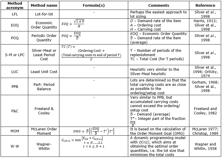
Perhaps the easiest approach to lot sizing is Lot-for-Lot (LFL), which simply requests the exact amount required for each time period. This approach is not cost effective when fixed replenishment costs (setup costs) are significant, because an order will have to be made for each time period (Silver et al., 1998).
When there is no variability in demand, the Harris’s EOQ method establishes the ideal size of the replenishment quantity (Harris, 1913). In general, there is variability in demand, in which case the results of the EOQ method are far from the desired, i.e. the optimum lot size strategy or the strategy that minimizes the production, inventory and setup costs. Therefore, there are two options, using heuristic or exact methods.
Heuristic methods are simple, but quite effective. Some of them present results very close to the optimal ones. The problem with heuristic techniques is the lack of information on the quality of the solutions; therefore, studies that compare the results of several heuristics to evaluate the quality of each technique are necessary.
Exact methods present the optimal result, but often fail to do so in a timely manner and may consume too many computational resources. Unlike complex algorithms, heuristics are simple and efficient techniques that can present acceptable results without intensive consumption of computational resources (calculation time).
In Karimi et al. (2003), the authors present an overview of exact and heuristic methods to approach the Capacitated Lot-sizing Problem (CLSP), Multi-Level Lot-sizing Problems without Resource Constraints (MLUR), and Multi-Level Lot-sizing Problems with Resource Constraints (MLCR), and the conclusion is that heuristic approaches are preferable. Meta-heuristics, such as SA (Simulated Annealing) or TS (Tabu Search), are also proposed as effective and efficient techniques to approach similar NP-hard problems. In Al-Salamah (2018), the author proposes a model to determine the optimal lot size of items of imperfect quality. Later he solved the model with ABC (Artificial Bee Colony), which has been shown to be an efficient meta-heuristic (Santos et al., 2016). Andriolo et al. (2014), examine the evolution of the lot size methods, from Harris’s EOQ to most of the state of the art lot-sizing techniques. In that paper, the authors also outline the future of lot-sizing models, which should take into consideration the social and environmental sustainability in the inventory management, as well as focus on closed-loop supply chains. Glock et al. (2014), reviewed the latest advances in lot-sizing techniques. First, the authors developed a classification scheme for lot-sizing models and then evaluated the extensions to Harris’s EOQ, such as lot-sizing models that consider scheduling issues, models that consider incentive systems and models that consider productivity issues. In that paper, the authors also demonstrated the popularity of the topic, with an increase in the number of the peer-reviewed papers published, predominantly in the last decade. Lastly, the authors presented several recommendations regarding future research about lot-sizing techniques and models. One variation of the single-item lot size problem, the Energy-Lot Size Problem (Energy-LSP), where it is necessary to decide which resources to use and how much to produce when machines have a limit in terms of how much energy can be consumed, is presented in Rapine et al. (2018).
The EOQ is one of the earliest and most well-known results of inventory theory, proposed by F. W. Harris in 1913. This method is also known as the Wilson’s lot size because R. H. Wilson was the one who initially applied this model in his consulting activities at several North American Companies. This model establishes a fixed order quantity that aims to minimize the total costs, i.e. carrying and ordering costs.
One recent extension to Harris’s EOQ is the incorporation of sustainability. In 2008, Turkay (2008) extended the EOQ to include environmental issues, which represent another cost. Other revisions to the Harris’s ECQ model that minimize the carbon emissions were proposed in Arslan and Turkay (2013), Benjaafar et al. (2010), and Hue et al. (2011). The Sustainable Economic Order Quantity (S-EOQ) model, which incorporates into the traditional EOQ model an LCA (Life Cycle Assessment) of the purchase or production order, was proposed by Battini et al. (2014). In that paper, the authors concluded that the difference between the EOQ and the proposed S-EOQ is minor, about 20% of the lot size, but it increases with the price of the product.
The Periodic Order Quantity (POQ) method contrasts with EOQ approach, which has irregular timing but constant quantities. In this method, the time interval in which the orders are going to be made is determined, and the quantity of the batch size must suppress the needs until the next order (Silver et al., 1998).
Another interesting heuristic was developed by Edward Silver e Harlan Meal (Silver and Meal, 1973), also known as the Least Period Cost (LPC). The Silver-Meal Heuristic selects the replenishment quantity that minimizes the total costs per unit time.
Usually this heuristic presents very good results, often close to the optimum. However, there are situations in which this heuristic can compromise (Silver et al., 1998):
It is important to notice that Edward Silver and John Miltenburg (1984) proposed a modified version of the Silver-Meal Heuristic (Silver et al., 1998) to cope with the heuristics underperformance when the forecast demands decreases rapidly or when there are extended periods without demand. In the computational study the authors were able to demonstrate the advantages of the modification, which do not increase the complexity of the heuristics.
The Least Unit Cost (LUC) heuristic is very similar to the Silver-Meal heuristic. The total costs are accounted for each period, considering the quantity of the replenishment, obtaining the total cost per unit. The costs per period are accumulated until the cost per unit is higher than the previous period (Orlicky, 1974; Silver et al., 1998).
In 1968, Gorham presented the Part-Period Balance heuristic, which basically consists on using the selection of the number of periods covered by the replenishment as a basic criterion, such that the total carrying costs are made as close as possible to the ordering/setup cost. The carrying costs per period are accumulated until the sum approaches or equals the ordering/setup cost (Gorham, 1968; Silver et al., 1998).
Another heuristic, developed in 1984, was proposed by Freeland & Cooley (F&C). This heuristic is very similar to the Part-Period Balance heuristic, with the exception that the accumulated carrying costs cannot exceed the ordering/setup cost (Freeland and Colley, 1982; Mukhopadhyay, 2015).
The procedure for the McLaren Order Moment (MOM) heuristic starts by the calculation of the Order Moment Goal (OMG) (McLaren, 1977). One overview of the MOM for multiple-purchase discounts is presented in Christoph (1989). In that paper, the author compares the MOM with four other lot-sizing techniques and concludes that the MOM is one of the best overall performers in multiple-purchase discounts in an MRP environment; however, it is not as simple to implement as the Silver-Meal heuristics or Lot-for-Lot.
The main idea underlying this procedure refers to the replenishment that should cover the periods 1 to k-1, when it is more economic to make a new order than keeping the stock of period k in inventory (McLaren, 1977; Meredith, 1992; Vollmann et al., 1992).
Wagner and Whitin (1958) introduced a method to solve the lot-sizing problem in O(n2) time. This method is a dynamic programming model that aims at obtaining the optimal order quantities, i.e. the lot size that minimizes the total costs. The computational work of the algorithm is reduced because the optimal solution must satisfy the following two properties:
The algorithm starts from the last period, N, and repeats itself until period 1. For each period t, it is selected the value of k which corresponds to the lowest total cost, i.e. the number of periods for which the order will be made in period t (Wagner and Whitin, 1958; Gonçalves, 2010). One exact method is presented in Wagelmans et al. (1992), and it can solve the problem in O(n log n) time and shows that the Wagner-Whitin case can be solved in linear time.
Many other lot-sizing methods do exist, and are constantly being put forward nowadays; however, the authors did just select these set of methods, as they are quite representative and continue to be widely used for establishing a different kind of analysis.
In Table 1, the previously shortly described information regarding the lot-sizing methods is summarized, for better clarification.
Table 1. Summary of lot-sizing methods
This work used a quantitative research methodology (Sanders, 1982) to analyze the behavior of a set of ten lot-sizing methods when applied to different application scenarios, with variations of demand and peaks in seasonality, to cover distinct real applications in manufacturing environments that can occur either in MRP or in JIT/ Kanban-oriented production systems. Figure 1 below illustrates the research methodology used, which includes five main steps.
Figure 1. Research methodology used.
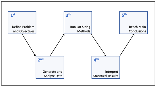
In the first step, the problem and corresponding objectives are defined: analyzing the behavior of a set of ten lot-sizing methods regarding its application on two different manufacturing environments, oriented to MRP and JIT/Kanban production philosophies, considering distinct application scenarios with variations on demand and peaks of seasonality. In step two, the data associated to the previously defined application scenarios, with variations in demand and peaks of seasonality, were generated and analyzed. In the third step, the heuristic lot-sizing methods were run for the different application scenarios defined, by using the corresponding generated data. In the fourth step, the results obtained through the execution of the heuristic lot-sizing methods were statistically analyzed. Finally, in step five, some main conclusions were extracted, regarding the analysis of the suitability of the different heuristic lot-sizing methods for being applied under different application scenarios, regarding variations in demand and peaks of seasonality, for MRP and JIT/Kanban-oriented manufacturing environments.
The lot-sizing methods referred above were tested through an original software prototype, which was developed using VBA programming language that is built in Microsoft Excel to expand the software functionalities, allowing the creation of user-defined functions and forms, including the handling of text boxes, buttons and other fully custom-made interaction features. Moreover, it contains the input data section where the user can input all the required data and the results section where the results are shown, and it has the option to output different reports. This kind of tool is of upmost importance in terms of academic support but also for companies, for instance regarding micro and small businesses (Galvão et al., 2017).
In this work, a study was carried out based on simulated data for 12 periods. Moreover, the ordering cost, unit cost, and the percentage holding cost per period was introduced, as data is required to run the methods. In the results section, the total costs, ordering costs, holding costs, and percentage error of total cost are shown to the nine heuristics and one exact method considered in this work.
The percentage error of the total was used to act as a benchmark based on the exact Wagner-Whitin method. This performance indicator is calculated through the difference between the heuristic and exact method total cost, in percentage.
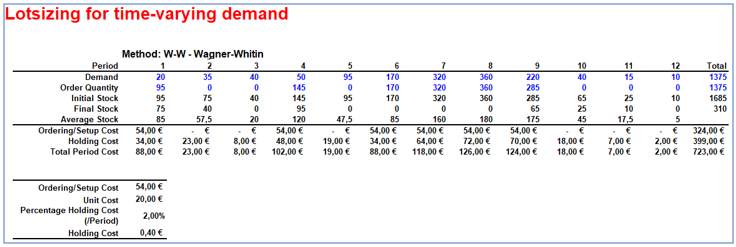
The “Report” buttons on results section generates a new worksheet with a detailed report with the solution for each selected method. The solution shows the order quantity which minimizes the overall cost. As shown in Figure 2, the report includes all the parameters considered on single-level lot-sizing problems with the discrimination of initial, average, and final stock, as well as ordering, holding, and total costs for each period.
To evaluate the performance of the heuristic methods in situations with different variation scenarios on demand, several distinct contexts were generated following a normal distribution, characterized by an average (µ) and standard deviation (σ) (Baciarello et al. 2013). The average demand value was defined as µ = 250 for each context or application scenario, and only the standard deviation varies from 10 ≤ σ ≤ 80 with an increment of 10. For each standard deviation, 100 different scenarios were tested.
Figure 2. Lot sizing detailed report for Wagner-Whitin method.
To evaluate the performance of the heuristic methods in situations with different seasonality effects, the scenarios were generated with different seasonality index, maintaining the average demand value of the series and the period of seasonality. The average was defined as µ = 250 and the seasonality index varies in the interval of [66;99;133;166;199;233]. For each seasonality index, 100 different scenarios were tested.
In all situations, the ordering cost was fixed at 150€, unit cost at 20€ and holding cost at 2% per period.
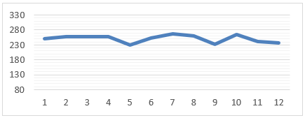
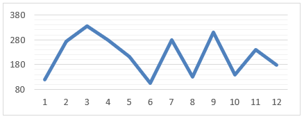
These scenarios are characterized with an average demand µ=250 and standard deviation σ=10. This scenario describes a simulated demand with very low variation as the example shown in Figure 3. This scenario represents, for example, the sales of consumer goods, such as toilet paper, shampoo or a very stable production in a flow shop or product-oriented manufacturing environment, for instance under JIT/Kanban manufacturing principles.
Figure 3. Example of a generated demand scenario for µ=250 and σ=10
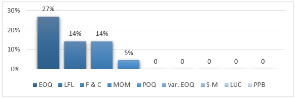
The results of the performance of the heuristic methods in scenario 1 are shown in Figure 4. In this scenario four heuristic methods were able to achieve the optimal result. The worst result belonged to EOQ, with 27% mean error in the total cost, compared to the optimal result.
Figure 4. Mean error in Total Cost for 100 scenarios with µ=250 and σ=10
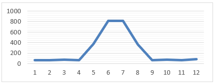
These scenarios are characterized by an average demand µ=250 and standard deviation σ=80. This type of variability in demand may be seen, for example, on a job shop manufacturing system, which deals with very different products and processes.
Figure 5. Example of a generated demand scenario for µ=250 and σ=80
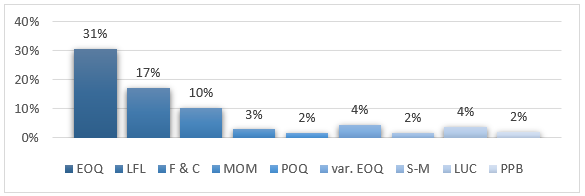
As shown in Figure 6, in general, the quality of the results decreases with the increase of standard deviation. However, some heuristics were able to achieve results close to the optimal solution, such as Silver-Meal, POQ and Part Period Balance, that achieved 2% error. The Freeland & Cooley and the MOM methods were the only ones that performed better than with low variation, and the worst result belonged once again to EOQ, with a 31% error.
Figure 6. Mean error in Total Cost for 100 scenarios with µ=250 and σ=80
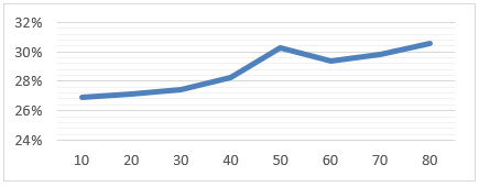
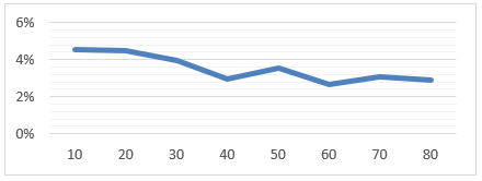
Demand variation influences directly the performance of the methods. As shown in Figure 7, the EOQ error increases with the increment of standard deviation. In this case, with standard variation σ = 10, the total cost error is 26.8% and increases consistently to 30.6% when σ = 80. This tendency is also applicable to LFL, POQ, var.EOQ, S-M, LUC, and PPB.
Figure 7. EOQ Performance with the increase of standard deviation in demand
However, this does not apply to Freeland & Cooley and MOM. The performance of these methods behaves in the opposite way to the previous ones. For example, the error of MOM decreased with the increment of standard deviation, as shown in Figure 8, as it goes from 4.5% when σ = 10 to 2.9% when σ = 80.
Figure 8. MOM Performance with the increase of standard deviation in demand
These scenarios are characterized by a seasonality index of 66 (Figure 9), a seasonal demand was simulated, with a moderate peak in demand for some periods, followed by a fall, in relation to to previous values.
Figure 9. Example of a generated demand scenario for µ=250 and seasonality index 66
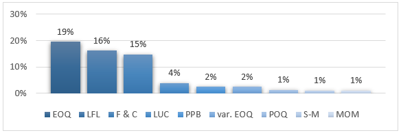
The results of the heuristic methods for seasonal demand scenarios are shown in Figure 10. In these scenarios none of the methods were able to achieve the optimal solution. The best result belonged to the POQ, Silver-Meal, and MOM, with 1% error when compared to the optimal result given by the Wagner-Whitin method. On the other side, the Lot-For-Lot method obtained an error of almost 16% and the Freeland & Cooley method obtained an error of 15%. Once again, EOQ obtained the worst result with an error of 19%.
Figure 10. Mean error in Total Cost for 100 scenarios with µ=250 and seasonality index 66
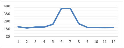
These scenarios are characterized by a seasonality index of 233 (Figure 11), a seasonal demand was simulated, with a high peak in demand for some periods, followed by a sharp fall to previous values.
Figure 11. Example of a generated demand scenario for µ=250 and seasonality index 233
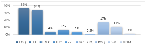
The results of the heuristic methods for the seasonal demand scenarios are shown in Figure 12. Once again, none of the methods were able to achieve the optimal solution. The best result was reached by the variable EOQ, with a 0.3% error when, compared to the optimal result. EOQ obtained the worst result with an error of 36%, followed by LFL with 34%. Freeland & Cooley tended to get better results than with lower seasonality index, opposed by POQ and S-M, which tended to achieve worst results.
Figure 12. Mean error in Total Cost for 100 scenarios with µ=250 and seasonality index 233
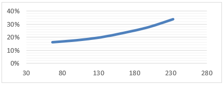
The performance variation with the increment of seasonality index is more irregular than with standard deviation. For LFL, POQ and S-M, with the increase of seasonality index, the error increased in a consistent and almost linear way. For example, as shown in Figure 13, the LFL error increased from 16% with Index=66 to 33.7% with index=233.
Figure 13. Performance of LFL with the increase of seasonality in demand
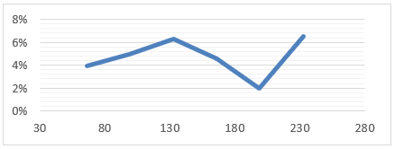
For EOQ, LUC, S-M, PPB, F&C, and MOM, the performance varies in an irregular way. In the example shown in Figure 14, LUC error changed its tendency twice with the increase of the seasonality index. This is also applicable to the previously referred methods.
Figure 14. LUC Performance with the increase of seasonality in demand
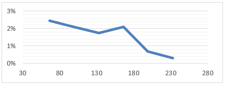
Variable EOQ was the only one that decreased its error with the increment of seasonality index. With index 33, variable EOQ performed a 2.4% error and decreased to 0.3% with index 233.
Figure 15. Performance of the variable EOQ with the increase of seasonality in demand
According to the results exposed and explained before, which are also summarized in Table 2, it is possible to realize that there are lot-sizing methods that performed worse than others regarding the increase in either demand variation or the seasonality index, as explained before, and the methods that performed worse in this regard are those that did present a higher error deviation, which were the EOQ, LFL, var.EOQ, and LUC, regarding increase in the demand variations, and EOQ, LFL, S-M, and LUC, in relation to the increase in the seasonality index.
Table 2. Summary of the errors deviations for lot-sizing methods regarding increases in demand variations and seasonality indexes.
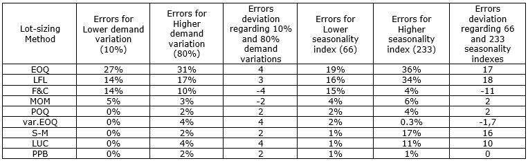
Through this information analysis it is possible to conclude that the methods EOQ, LFL, var-EOQ, and LUC clearly present higher application risk in scenarios marked by a considerable deviation in demand, and the methods EOQ, LFL, S-M, and LUC, regarding an increase in seasonality peaks, which typically occur more frequently in the context of MPR-based manufacturing contexts, associated with higher variation of materials, lot sizes or orders batches, and are typically produced in function or process-oriented manufacturing systems. Therefore, the application of these methods may be avoided in these kinds of manufacturing environments, as they may allow obtaining good results or solutions in these kinds of application scenarios.
On the other hand, it is also possible to conclude that these lot-sizing methods can be better suited for being applied in JIT/Kanban production scenarios, as this kind of underlying manufacturing environment is characterized by typically having a more stable demand.
Moreover, all the remaining lot-sizing method, which did perform better or even very well either regarding increasing the demand variations or seasonality indexes, could thus be appropriately suited for being applied either in MRP or JIT/Kanban based manufacturing environments.
The results obtained through this work showed that, in fact, some heuristic methods can produce results very close to the optimal one, even when the demand data has high variability on it. In the three simulated application scenarios presented, it was possible to notice that several heuristics obtained consistent results with percentage errors of less than 5%. With low variation in demand, several heuristics were able to achieve optimal results, and with high variation, the best heuristics were POQ, S-M, and PPB, with a 2% error.
On the other hand, the EOQ method always presented high percentage errors, even in scenarios with lower variability in the demand data, which allows concluding, through the results obtained, that heuristic methods are a good option, in general, regarding demand variations and seasonality peak analysis.
Standard deviation influences the performance of heuristics. For EOQ, LFL, POQ, var.EOQ, M-S, LUC, and PPB, the increase of standard deviation results in an increased error from optimal solution. This is a consistent trend in the results of the methods. For F&C and MOM, an increase in the standard deviation results in a decreased error from the optimal solution.
In scenarios with seasonality, the increase of the seasonality index resulted in worse results in almost all methods, except for F&C, var.EOQ, and MOM. In fact, F&C achieved much better results with higher seasonality, with a drop from 15% to 4% error, and var.EOQ achieved 0.3% error in high seasonality scenarios. Moreover, with an increase of seasonality in demand, heuristics behavior tends to become more irregular.
All results were obtained using generated scenarios, with specific conditions for ordering and holding costs, and not with real situations. In this paper, an analysis based on different scenarios of application of the lot-sizing methods studied regarding situations about variation in demand and peaks of seasonality was presented. Afterwards, an extended analysis of the suitability of the considered heuristic lot-sizing methods was performed under different manufacturing and management philosophies in relation to the more traditional MRP-based systems and those based on the JIT/Kanbans principles. Therefore, through this study it was possible to conclude that the methods EOQ, LFL, var.EOQ, and LUC presented higher risk of application in scenarios marked by a considerable deviation in demand, and methods such as EOQ, LFL, S-M, and LUC, regarding an increase in peaks of seasonality, which are situations that typically occur more frequently in the context of MPR-based manufacturing environments, thus being better suited for application in the JIT/Kanban production scenarios, as this kind of underlying manufacturing context is characterized by typically having a more stable demand.
Summarizing, the results obtained show that some lot-sizing methods are better suited than others to be applied in specific scenarios marked by a considerable variation in demand or peaks of seasonality. Thus, this research contributes to further clarify industrial practitioners on the selection of the best suited lot-sizing methods for each type of application scenario regarding MRP or JIT/ Kanban manufacturing environments.
In terms of future work, additional analysis on the lot-sizing methods will be carried out to further evaluate the strengths and weaknesses of different methods under different types of scenarios, for instance to analyze its performance according to variations in the ordering and stock holding costs.
This work has been supported by FCT - Fundação para a Ciência e Tecnologia within the Project Scope: UID/CEC/00319/2019.
Al-Salamah, M. (2018), “Economic production quantity with the presence of imperfect quality and random machine breakdown and repair based on the artificial bee colony heuristic”, Applied Mathematical Modelling, Vol. 63, pp. 68–83.
Andriolo, A. et al. (2014), “A Century of Evolution from Harris’s Basic Lot Size Model: Survay and Research Agenda”, International Journal of Production Economics, Vol. 155, pp. 16-38.
Ani, C. et al. (2018), “Analysis of the effective production Kanban size with triggering system for achieving just-in-time (JIT) production”, In 2018 4th International Conference on Control, Automation and Robotics (ICCAR), pp. 316-320, IEEE.
Araújo, M. et al. (2017), “Improving Productivity and Standard Time Updating in an Industrial Company–A Case Study”, In International Conference of Mechatronics and Cyber-Mixmechatronics, pp. 220-228, Springer.
Araújo, S. A. (1999), Estudos de problemas de dimensionamento de lotes monoestágio com restrição de capacidade, Dissertação de Mestrado em Ciências, Universidade de São Paulo, São Carlos, SP.
Arslan, M., Turkay, M. (2013), “EOQ Revisited with Sustainability Considerations”, Foundations of Computing and Decision Sciences, Vol. 38, pp. 223-249.
Baciarello L. et al. (2013), “Lot Sizing Heuristics Performance”, International Journal of Engineering Business Management, Vol. 5. DOI: 10.5772/56004
Battini, D. et al. (2014), “A Sustainable EOQ Model: Theoretical Formulation and Applications”, International Journal of Production Economics, Vol. 149, pp. 145-153.
Behnamian, J. et al. (2017), “A Markovian approach for multi-level multi-product multi-period capacitated lot-sizing problem with uncertainty in levels”, International Journal of Production Research, Vol. 55, No. 18, pp. 5330-5340.
Benjaafar, S. et al. (2010), “Carbon Footprint and the Management of Supply Chains: Insights from Simple Models”, IEEE Transactions on Automation Science and Engineering, Vol. 10, No. 1, pp. 99-116.
Chase, R. B. et al. (2006), Operations Management for Competitive Advantage, 11th Edition, Irwin, McGraw Hill.
Chiarini, A. (2017), “An adaptation of the EOQ formula for JIT quasi-pull system production”, Production Planning & Control, Vol. 28, No. 2, pp. 123-130.
Christoph, O. B. (1989), “McLaren’s Order Moment Lot-Sizing Technique in Multiple Discounts”, Production and Inventory Management Journal, Vol. 30, No. 2, pp. 44-48.
Freeland, J. R.; Colley J. L. (1982), “A Simple Heuristic Method for Lot Sizing in a Time‐Phased Reorder System”, Production and Inventory Management, Vol. 23, No. 1, pp. 15‐21.
Galvão, E. M. et al. (2017), “Sales Performance Management: A Strategic Initiative to the Growth of Micro and Small Businesses”, Brazilian Journal of Operations & Production Management, Vol. 14, No. 1, pp. 118-124.
Glock, C. H. et al. (2014), “The Lot Sizing Problem: A Tertiary Study”, International Journal of Production Economics, Vol. 155, pp. 39-51.
Gonçalves, J. (2010), Gestão de Aprovisionamentos, 2nd Edition, Publindústria, Porto.
Gorham T. (1968), “Dynamic Order Quantities”, Production and, Inventory Management, Vol. 9, No. 1, pp. 75–79.
Goyal, S. K.; Gopalakrishnan, M. (1993), “A Comment On: A note on the EOQ-JIT Relationship”, Production Planning & Control, Vol. 4, No. 3, pp. 283–285.
Gu, Q. et al. (2017), “Exploiting timely demand information in determining production lot-sizing: an exploratory study”, International Journal of Production Research, Vol. 55, No. 16, pp. 4531-4543.
Harris, F.W. (1913), “How Many Parts to Make at Once”, The Magazine of Management, Vol. 10, pp. 135‐136.
Hue, G. et al. (2011), “Managing Carbon Footprints in Inventory Management”, International Journal of Production Economics, Vol. 131, pp. 313-321.
Jamal, A. M. M.; Sarker, B. R. (1993), “An Optimal Batch Size for a Production System Operating Under a Just-In-Time Delivery System”, International Journal of Production Economics, Vol. 32, No. 2, pp. 255-260.
Karimi, B. et al. (2003), “The Capacitated Lot Sizing Problem: A Review of Models and Algorithms”, Omega - The International Journal of Management Science, Vol. 31, pp. 365-378.
Kuo, W. H. (2005), “An Analytical Comparison of Inventory Costs of JIT and EOQ Purchasing with Defective Products”, Journal of Information and Optimization Sciences, Vol. 26, No. 1, pp. 219-231.
Li, H.; Thorstenson, A. (2014), “A multi-phase algorithm for a joint lot-sizing and pricing problem with stochastic demands”, International Journal of Production Research, Vol. 52, No. 8, pp. 2345-2362.
Marques, M. S. (2013), O Problema do Sequenciamento e Dimensionamento de Lotes no Planeamento da Produção, Dissertação de Mestrado em Engenharia e Gestão Industrial, Universidade da Beira Interior, Covilhã.
Masmoudi, O. et al. (2017), “Lot-sizing in a multi-stage flow line production system with energy consideration”, International Journal of Production Research, Vol. 55, No. 6, pp. 1640-1663.
McLaren, B. J. (1977), “A Study of Multiple Level Lot Sizing Procedures for Material Requirements Planning Systems”, PhD dissertation, Purdue University.
Meredith, J. R. (1992), The Management of Operations: A Conceptual Emphasis, John Wiley & Sons, Inc, New York.
Miclo, R. et al. (2015), “MRP vs. demand-driven MRP: Towards an objective comparison”, In 2015 International Conference on Industrial Engineering and Systems Management (IESM), Seville, Spain, 21-23 Oct., pp. 1072-1080. DOI: 10.1109/IESM.2015.7380288
Miclo, R. et al. (2018), “Demand Driven MRP: assessment of a new approach to materials management”, International Journal of Production Research, Vol. 57, No. 1. DOI: 10.1080/00207543.2018.1464230
Moily, J. P. (2015), “Economic Manufacturing Quantity and Its Integrating Implications”, Production and Operations Management, Vol. 24, No. 11, pp. 1696-1705.
Mukhopadhyay, S. K. (2015), Production Planning and Control – Text and Cases, 3rd Edition, Phi Learning Private Limited, Delhi.
Nunes, D. R. L.; Vieira, A. F. C. (2016), “An Inventory Model for Optimization of a Two-Echelon Periodic-Review System”, Brazilian Journal of Operations & Production Management, Vol. 13, No. 1, pp. 2-15.
Orlicky J. (1974), Material Requirements Planning, McGraw Hill, New York.
Rabbani, M. et al. (2017), “Capacity coordination in hybrid make-to-stock/make-to-order contexts using an enhanced multi-stage model”, Brazilian Journal of Operations & Production Management, Vol 14, No. 3, pp. 396-413.
Rapine, C. et al. (2018), “Capacity Acquisition for the Single-Item Lot Sizing Problem Under Energy Constraints”, Omega, Vol. 81, pp. 112-122.
Salgado, P.; Varela, L. (2010), “Kanban Sharing and Optimization in Bosch Production System”, KMIS, pp. 81-91. DOI: 10.5220/0003102600810091
Sanders, P. (1982), “Phenomenology: A new way of viewing organizational research”, Academy of Management Review, Vol. 7, No. 3, pp. 353-360.
Santos, A. S. et al. (2016), “Evaluation of the Simulated Annealing and the Discrete Artificial Bee Colony in the Weight Tardiness Problem with Taguchi Experiments Parameterization”, Advances in Intelligent Systems and Computing, Vol. 557, pp. 718–727.
Silva, C. et al. (2017), “A comparison of production control systems in a flexible flow shop”, Procedia Manufacturing, Vol. 13, pp. 1090-1095.
Silver E. A.; Meal H. C. (1973), “A Heuristic Selecting Lot Size Requirements for the Case of a Deterministic Time Varying Demand Rate and Discrete Opportunities for Replenishment”, Production and Inventory Management, Vol. 14, No. 2, pp. 64‐74.
Silver, E. A. et al. (1998), Inventory Management and Production Planning and Scheduling, 3rd Edition, John Wiley & Sons, New York.
Silver, E. A., Miltenburg, J. (1984), “Two Modifications of the Silver-Meal Lot Sizing Heuristic”, INFOR: Information Systems and Operational Research, Vol. 22, pp. 55-69.
Turkay, W. (2008), “Environmentally Conscious Supply Chain Management”, Process System Engineering: Supply Chain Optimization, Vol. 3, pp. 45-86.
Varela, M. L. et al. (2018), “Collaborative paradigm for single-machine scheduling under just-in-time principles: total holding-tardiness cost problem”, Management and Production Engineering Review, Vol. 9. DOI:10.24425/119404
Vollmann T. E. et al. (1992), Manufacturing Planning and Control Systems, 3rd Edition. Richard D. Irwin, Inc.
Vörös, J.; Rappai, G. (2016), “Process quality adjusted lot sizing and marketing interface in JIT environment”, Applied Mathematical Modelling, Vol. 40, pp. 6708–6724.
Wagelmans, A. et al. (1992), “Economic Lot Sizing: An O(n log n) Algorithm that Runs in Linear Time in the Wagner-Whitin Case”, Operations Research, Vol. 40, pp. 145-156.
Wagner H. M., Whitin T. M. (1958), “Dynamic Version of the Economic Lot Size Model”, Management Science, Vol. 5, No. 1, pp. 89‐96.
Wang, H. et al. (2017), “Information processing structures and decision making delays in MRP and JIT”, International Journal of Production Economics, Vol, 188, pp. 41-49.
Received: 18 May 2018
Approved: 22 Mar 2019
DOI: 10.14488/BJOPM.2019.v16.n4.a9
How to cite: Florim, W.; Dias, P.; Santos, A. S. et al. (2019), “Analysis of lot-sizing methods’ suitability for different manufacturing application scenarios oriented to MRP and JIT/Kanban environments”, Brazilian Journal of Operations & Production Management, Vol. 16, No. 4, pp. 638-649, available from: https://bjopm.emnuvens.com.br/bjopm/article/view/497 (access year month day).