Optimization using evolutionary metaheuristic techniques: a brief review
Aparna Chaparala
chaparala_aparna@yahoo.com
Dept of CSE, RVR&JC College of Engineering (A), Guntur, AP
Radhika Sajja
sajjar99@yahoo.com
Dept of ME, RVR&JC College of Engineering (A), Guntur, AP
ABSTRACT
Optimization is necessary for finding appropriate solutions to a range of real life problems. Evolutionary-approach-based meta-heuristics have gained prominence in recent years for solving Multi Objective Optimization Problems (MOOP). Multi Objective Evolutionary Approaches (MOEA) has substantial success across a variety of real-world engineering applications. The present paper attempts to provide a general overview of a few selected algorithms, including genetic algorithms, ant colony optimization, particle swarm optimization, and simulated annealing techniques. Additionally, the review is extended to present differential evolution and teaching-learning-based optimization. Few applications of the said algorithms are also presented. This review intends to serve as a reference for further work in this domain.
Keywords: Optimization; Evolutionary algorithms; Meta-heuristic techniques; Applications.
1 INTRODUCTION
Automation in manufacturing industry has been witnessing the rapid applications of Computational Intelligence (CI) (Mackworth et Goebel, 1998) for a decade. The growing complexity of computer programs, availability, increased speed of computations, and their ever-decreasing costs have already manifested a momentous impact on CI. Amongst the computational paradigms, Evolutionary Computation (EC) (Kicinger et al., 2005) is currently apperceived all over. Unlike the static models of hard computing, which aim at identifying the properties of the problem being solved, the EC comprises a set of soft-computing paradigms (Schwefel, 1977). The word paradigm, here, should be understood as an algorithm that underlines the computational procedure to find an optimal solution to any given problem. Objectives of optimization implicitly include reducing computational time and complexity. For this very reason, competing methods of optimization have grown over the years. However, over time, each method—traditional or modern—has found specific applications. Evolutionary computational methods are metaheuristics that are able to search large regions of the solution's space without being trapped in local optima.
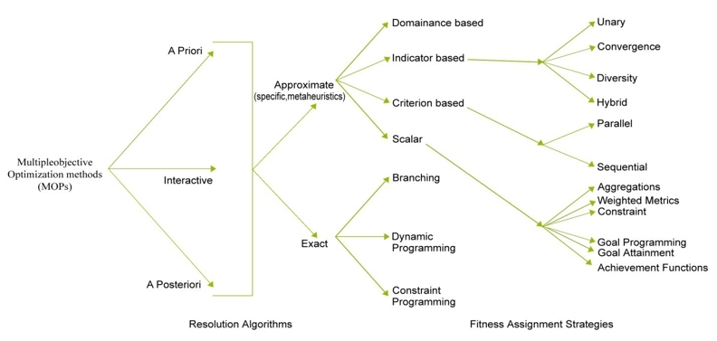
The single-criterion optimization problem has a single optimization solution with a single objective function. In a multi-criterion optimization firm, there is more than one objective function, each of which may have an uncooperative self-optimal decision. Multi-objective Optimization Problems (MOPs) are the crucial areas in science and engineering. The complexity of MOPs depends on the size of the problem to be solved, i.e. the complexity is significantly affected by the number of objective functions and size of the search space (Jain et al., 1999) . Figure 1 depicts the broad classification of MOP.
Figure 1. Taxonomy of MOPs
In general, all CI algorithms developed for optimization can be categorized as deterministic or stochastic. The former type use gradient techniques and can be more appropriately used in solving unimodal problems. The later can further be classified as heuristic and meta-heuristic models. The difficulty in terms of optimization of engineering problems has given way to the development of an important heuristic search algorithmic group, namely, the Evolutionary Algorithm group. Meta-heuristics techniques comprise a variety of methods including optimization paradigms that are based on evolutionary mechanisms, such as biological genetics and natural selections.
As indicted by Rao et al. (Rao et al., 2011) optimization of large scale problems is often associated with many difficulties, such as multimodality, dimensionality and differentiability. Traditional techniques as linear programming, dynamic programming, etc. generally fail to solve such large scale problems, especially with non-linear objective functions. As most of these require gradient information, it is not possible to solve non-differentiable functions with the help of such techniques. In addition, the following limitations are observed in traditional optimization techniques:
• Traditional optimization techniques start with a single point.
• The convergence to an optimal solution depends on the chosen initial random solution.
• The results tend to stick with local optima.
• Are not efficient when practical search space is too large and follow a deterministic rule.
• Are not efficient in handling the multi-objective functions.
• Optimal solutions obtained are applicable to problems of very small size.
• Require excessive computation time and are not practical for use on a daily basis.
• Also, modeling the techniques is a difficult task.
These limitations urge the researchers to implement metaheuristic techniques in application domains. Scheduling problems are proved to be NP-hard types of problems and are not easily or exactly solved for large sizes. The application of metaheuristics technique to solve such NP hard problems needs attention. A futile effort that this paper will not pursue is to overstate the capabilities of the optimization methods discussed herein. Rather, the objective is to present how population-based meta-heuristic techniques work and indicate their applications. This paper goes on to present, in the following sections, genetic algorithms, ant colony optimization, particle swarm optimization, simulated annealing, differential evolution, and teaching-learning-based optimization, and the conclusion.
2 META-HEURISTIC OPTIMIZATION
A meta-heuristic is described as an iterative master process that guides and modifies the operations of subordinate heuristics to efficiently produce high quality solutions (Osman et Laporte, 1996). It may manipulate a complete or incomplete single or a collection of solutions for every iteration. The subordinate heuristics may be high or low level procedures, or a simple local search or just a construction method. The meta-heuristics are not designed specifically for a particular problem, but are considered general approaches that can be tuned for any problem.
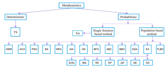
While solving optimization problems, single-solution-based metaheuristics improves a single solution in different domains. They could be viewed as walk-through neighborhoods or search trajectories through the search space of the problem. The walks are performed by iterative dealings that move from the present answer to a different one within the search area. Population-based metaheuristics (Ghosha et al., 2011) share the same concepts and are viewed as an iterative improvement in a population of solutions. First, the population is initialized. Then, a new population of solutions is generated. It is followed by generation for a replacement population of solutions. Finally, this new population is built-in into the present one using some selection procedures. The search method is stopped once a given condition is fulfilled. Figure 2 provides the taxonomy frameworks of multi-objective metaheuristics.
Figure 2. Taxonomy frameworks of meta-heuristics
Metaheuristics techniques comprise a variety of methods including optimization paradigms that are based on evolutionary mechanisms, such as biological genetics and natural selections. A metaheuristic is described as an iterative master process that guides and modifies the operations of subordinate heuristics to efficiently produce high quality solutions. It may manipulate a complete or incomplete single or a collection of solutions for every iteration. The subordinate heuristics may be high or low level procedures, or a simple local search or just a construction method. The metaheuristics that are not designed specifically for a particular problem but are considered general approaches that can be tuned for any problem.
While these methods provide many characteristics that make it the method of choice for the researchers in problem domain, the most important reasons are: the paradigms use direct ‘fitness’ information instead of functional derivatives and use probabilistic, rather than deterministic transition rules. This overcomes the problem of getting stuck in local optima prevalent with deterministic rules. There are several possible classifications for metaheuristics; however, one is commonly used in single solution approaches and population-based approaches. Single solution methods are Basic Local Search, Tabu Search, Simulated Annealing, Variable Neighborhood search, and others. Population-based methods include Genetic algorithm, Particle swarm optimization, Ant colony optimization, Scatter search, Memetic algorithm etc.
2.1 GENETIC ALGORITHM (GA)
David Goldberg (Goldberg, 1989) defined GA as: Genetic algorithms are the search algorithms based on the mechanics of natural selection and natural genetics. GA combines the survival of fitness among the string structure with structured, yet randomized information exchanges to form a search algorithm with some of the innovative flair of human search.
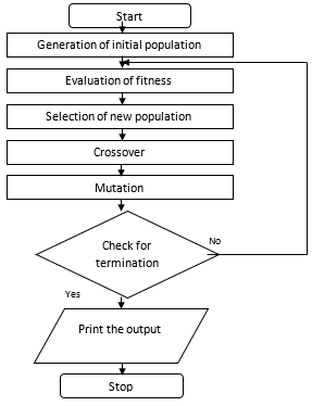
Genetic and Darwinian inheritance strive for survival. Each cell of every organism of a given species carries a certain number of chromosomes. Chromosomes are made of units of genes that are arranged in a linear succession. Every gene controls the inheritance of one or several characters. Genes of certain characters are located at certain places of the chromosome that are called string positions. Each chromosome would represent a potential solution to a problem. An evaluation process run on a population of chromosomes corresponds to a search through a space of potential solutions. Such a search requires balancing two objectives, namely, Exploiting the best solution and Exploring the search space. The steps of genetic algorithm are described below and the flowchart is shown in Figure 3.
Step 1: Generate random population of n chromosomes.
Step 2: Evaluate the fitness f(x) of each chromosome x in the population.
Step 3: Create a new population by repeating following steps until the new population is complete.
Step 4: Select two parent chromosomes from a population according to the fitness.
Step 5: With a crossover probability, crossover the parents to form a new offspring (Children). If no crossover was performed, offspring is an exact copy of parents.
Step 6: With a mutation probability, mutate new offspring at each position in chromosome.
Step 7: Place new offspring in a new population.
Step 8: Use new generated population for a further run of algorithm.
Step 9: If the end condition is satisfied, stop and return the best solution in current population and go to step 2.
Figure 3. Flowchart for genetic algorithm
2.2 SIMULATED ANNEALING ALGORITHM (SA)
Kalyanmoy (2002) defined SA algorithm as the method that resembles the cooling process of molten metals through annealing. At high temperatures, the atoms in the molten metal can move freely with respect to each other; however, as the temperature is reduced, the movement of atoms gets restricted. The atoms start to get ordered and finally form crystals having the minimum possible energy. Nonetheless, the formation of the crystal depends on the cooling rate. If the temperature is reduced at a faster rate, the crystalline state may not be achieved at all; instead, the system may end up in a polycrystalline state, which may have a higher energy state than the crystalline state. Therefore, to achieve the absolute minimum state, the temperature needs to be reduced at a slow rate. The process of slow cooling is known as annealing in metallurgical parlance. SA simulates this process of slow cooling of molten metal to achieve the minimum function value in a minimization problem. The cooling phenomenon is simulated by controlling a temperature as a parameter introduced with the concept of the Boltzmann probability distribution. According to the Boltzmann probability distribution, a system in thermal equilibrium at a temperature T has its energy distributed probabilistically, according to the equation (1).

Where k is the Boltzmann constant. This expression suggests that a system at a high temperature has almost uniform probability of being at any energy state; however, at a low temperature it has a small probability of being at a high energy state. Therefore, by controlling the temperature T and assuming that the search process follows the Boltzmann probability distribution, the convergence of an algorithm is controlled using the metropolis algorithm.
At any instant, the current point is x(t) and the function value at that point is E(t) = f(x(t)). Using the metropolis algorithm, the probability of the next point being at x(t+1) depends on the difference in the function values at these two points or on ΔE=E(t+1)-E(t) and is calculated using the Boltzmann probability distribution equation (2).

If ΔE ≤ 0, this probability is one and the point x(t+1) is always accepted. In the function minimization context, this makes sense because if the function value at x(t+1) is better than that at x(t), the point x(t+1) must be accepted. When ΔE> 0, it implies that the function value at x(t+1) is worse than that at x(t). According to the metropolis algorithm, there is some finite probability of selecting the point x(t+1) even though it is a worse than the point x(t). However, this probability is not the same in all situations. The probability depends on the relative magnitude of ΔE and T values. If the parameter T is large, this probability is more or less high for points with largely disparate function values. Thus, any point is almost acceptable for a large value of T. For small values of T, the points with only small deviation in function value are accepted. The steps of SA algorithm are described below and the flowchart is shown in Figure 4.
Figure 4. Flowchart for SA algorithm
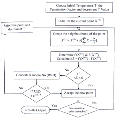
Step 1: Choose an initial point x (0), a termination criterion ε. Set T as a sufficiently high value, number of iterations to be performed at a particular temperature n and set t=0.
Step 2: Calculate a neighboring point x (t+1)=N(x (t) ) . Usually, a random point in the neighborhood is created.
Step 3: If ΔE = E(x (t+1) )- E(x (t) )< 0, set t = t +1; Else create a random number (r) in the range (0,1). If r ≤ exp (-ΔE/kT), set t = t + 1; Else goto step 2.
Step 4: If (x (t+1) - x (t) ) < ε and T is small, Terminate; Else go to Step 2.
2.3 ANT COLONY OPTIMIZATION ALGORITHM (ACO)
Ant algorithms were proposed by Dorigo and Gambardella (1997) as a multi-agent approach to different combinatorial optimization problems. The ant system is a new kind of co-operative search algorithm inspired by the behavior of colonies of real ants. The blind ants are able to find astonishing good solutions to the shortest path problems between food sources and home colony. The medium used to communicate information among individuals regarding paths, and decide where to go, was the pheromone trials. A moving ant lays some pheromone on the moving path, thus marking the path by the substance. While an isolated ant moves essentially at random, it can encounter a previously laid trail and decide with high probability to follow it, and also reinforcing the trail with its own pheromone. The collective behavior that emerges in a form of autocatalytic behavior, where the more the ants following a trail, the more attractive that trail becomes for being followed. There is a path along that ants are walking from nest to the food source and vice versa. If a sudden obstacle appears and the path is cut off, the choice is influenced by the intensity of the pheromone trails left by proceeding ants. On the shorter path more pheromone is laid down.
The ant colony optimization algorithm can be applied for the continuous function optimization algorithm. Hence, the domain has to be divided into a specific number of R randomly distributed regions. These regions are indeed the trial solutions and act as local stations for the ants to move and explore. The fitness of these regions are first evaluated and sorted on the basis of fitness. A population of ants totally explores these regions; the updating of the regions is done locally and globally with the local search and global search mechanism respectively. The steps of an ACO algorithm are described below and the flowchart is shown in Figure 5.
Figure 5. Flowchart for an ACO algorithm
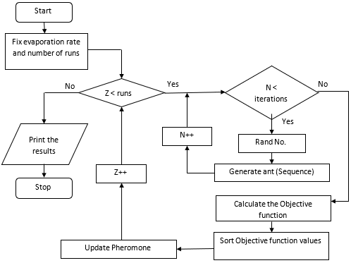
Step 1: Fix the evaporation rate and number of runs.
Step 2: While (number of runs is less than required).
Step 3: Initialize pheromone values.
Step 4: Call random number generation function.
Step 5: Generate group of ants with different paths.
Step 6: Call the function for calculating the objective function.
Step 7: Sort the objective function values in ascending order.
Step 8: For best sequences, update pheromone level.
Step 9: Repeat steps 4,5,6,7 and 8 till obtaining required number of runs.
Step 10: Print the best sequences and the objective function value.
Step 11: Change evaporation rate and number of runs for next trail.
2.4 PARTICLE SWARM OPTIMIZATION ALGORITHM (PSO)
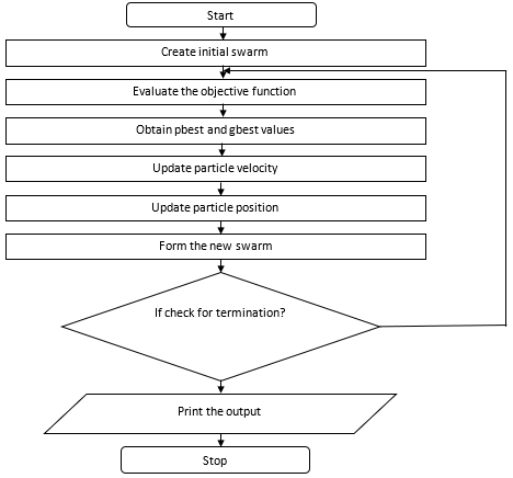
A swarm of individuals exploring a large solution space can benefit from sharing the experiences gained during the search with the other individuals in the population. This social behavior has inspired the development of Particle Swarm Optimization. PSO is an evolutionary computation technique developed by Kennedy and Eberhart in 1995. Similar to Genetic algorithm (GA), PSO is a population-based optimization tool, has fitness values to evaluate the population, and update the population for the optimum with random techniques. However, unlike GA, PSO has no evolution operators such as crossover and mutation (Kennedy et Ebehart, 1995). In PSO, particles update themselves with the initial velocity. In this algorithm, the individuals are not selected to survive or die in each generation. Instead all the individuals learn from the others and adapt themselves by trying to imitate the behavior of the fittest individuals. The PSO methods adhere to the basic principles of swarm intelligence like proximity, quality, diverse response, stability, and adaptability. The steps of PSO algorithm are described below and the flowchart is shown in Figure 6
Step 1: Initialize a population of ‘n’ particles randomly.
Step 2: Calculate fitness value for each particle. If the fitness value is better than the best fitness value (pbest) in history, then set current value as the new pbest.
Step 3: Choose particle with the best fitness value of all the particles at the gbest.
Step 4: For each particle, calculate particle velocity according to the equation (3) and equation (2.4).
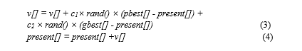
where v[] is the particle velocity
present[] is the current particle (solution)
pbest[] and gbest[] are defined as stated before
rand() is a random number between 0 and 1.
c1, c2 are learning factors. Usually c1 equals to c2 and ranges from 0 to 4.
Step 5: Particle velocities on each dimension are clamped to a maximum velocity V max. If the sum of acceleration would cause the velocity on that dimension to exceed V max (specified by the user), the velocity on the dimension is limited to V max.
Figure 6. Flowchart for PSO algorithm
2.5 DIFFERENTIAL EVOLUTION ALGORITHM (DE)
A simple, yet powerful, population-based stochastic search technique, Differential Evolution (DE) is first described by Price and Storn (1995) in the ICSI technical report. Since its invention, DE has been applied with high success on many numerical optimization problems (Lin et al., 2004; Cheng et Hwang, 2001). Due to its simplicity, ease in implementation and quick convergence, the DE algorithm has gained much attention and a wide range of successful applications (Onwubolu et Davendra, 2006; Qian et al., 2008). However, due to its continuous nature, the applications of DE algorithm that are used to solve production scheduling problems are still very limited (Tasgetiren et al., 2007).
2.5.1 Basics of Differential Evolution procedure
All evolutionary algorithms aim to improve the existing solution using the techniques of mutation, recombination and selection. The general paradigm of Differential Evolution is shown in Figure 7.
Figure 7. Differential Evolution algorithm scheme
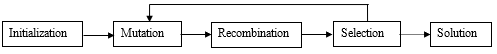
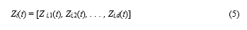
Initialization- Creation of a population of individuals. The ith individual vector (chromosome) of the population at current generation t with d dimensions is as follows,
Mutation - A random change of the vector Zi components. The change can be a single-point mutation, inversion, translocation, deletion, etc. For each individual vector Z k(t) that belongs to the current population, a new individual, called the mutant individual, U is derived through the combination of randomly selected and pre-specified individuals.
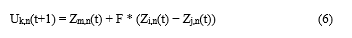
The indices m, n, i, and j are uniformly random integers mutually different and distinct from the current index ‘k’ and F is a real positive parameter, called mutation factor or scaling factor (usually Є [0, 1]).
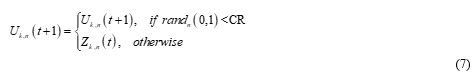
Recombination (Crossover) - merging the genetic information of two or more parent individuals for producing one or more descendants. DE has two crossover schemes, namely, the exponential crossover and the binomial or uniform crossover. Binomial crossover is used in the present work. The binomial or uniform crossover is performed on each component n (n= 1, 2, . . . , d) of the mutant individual U k,n (t+1). For each component a random number ‘r’ in the interval [0, 1] is drawn and compared with the Crossover Rate (CR) or recombination factor (another DE control parameter), CR Є [0, 1]. If r < CR, then the n th component of the mutant individual U k,n (t) will be selected; otherwise, the n th component of the target vector Z k,n (t) becomes the n th component.
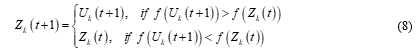
Selection - Choice of the best individuals for the next cycle. If the new offspring yields a better value of the objective function, it replaces its parent in the next generation; otherwise, the parent is retained in the population, i.e.
Where f ( ) is the objective function to be minimized.
2.5.2 Different mutation strategies of Differential Evolution
Different working strategies of DE are suggested by Storn and Price (1997) along with the guidelines for the application of these strategies to solve a problem. The strategies are represented as DE/x/y/z, where x is the vector, y is number of vectors whose difference is considered for mutation and z is the crossover scheme. ‘x’ takes either ‘rand’ or ‘best’ based on whether the vector is chosen randomly or the best one is chosen. ‘y’ takes either 1 or 2, to denote a single or two vector differences to be used for mutation. The index z takes either binomial (bin) or exponential (exp) based on the type of crossover scheme.
2.6 TEACHING-LEARNING-BASED OPTIMIZATION ALGORITHM (TLBO)
Teaching-Learning-Based Optimization (TLBO) algorithm, developed by Rao et al., is based on the natural phenomenon of teaching and learning process in a classroom (Rao et Kalyankar, 2010; Rao et al., 2011). TLBO does not require any algorithm specific parameters. In optimization algorithms, the population consists of different design variables. In TLBO, different design variables will be analogous to different subjects offered to learners and the learners’ result is analogous to the value of the fitness function, as in other population-based optimization techniques. The teacher is considered as the best solution in that particular generation. The process of working of TLBO is divided into two parts. The first part consists of ‘Teacher Phase’ and the second part consists of ‘Learner Phase’. The ‘Teacher Phase’ means learning from the teacher and the ‘Learner Phase’ means learning through the interaction between learners.
2.6.1 Teacher phase
Ideally good teachers bring their learners up to their level in terms of knowledge. In practice, this is not possible and a teacher can only move the mean of a class up to some extent, depending on the capability of the class. This follows a random process depending on many factors.
Initialization
The class X is randomly initialized by a given data set of n rows and d dimensions using the following equation.

The i th learner of the class X at the current generation t with d subjects is as follows,

The mean value of each subject, j, of the class in generation t is given as

The teacher is the best learner, X best with minimum objective function value in the current class. The Teacher phase tries to increase the mean result of the learners and always tries to shift the learners towards the teacher. A new set of improved learners can be generated from the Equation 3.22.

T F is the teaching factor with value between 1 and 2, and ‘r’ is the random number in the range [0, 1]. The value of T F can be found using the following equation:
2.6.2 Learner phase
Learners increase their knowledge by two different methods: one through input from the teacher and the other through interaction between themselves.
A learner learns something new if the other learner has more knowledge than him or her. For a learner ‘i’, another learner ‘j’ is randomly selected from the class.
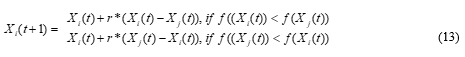
Where f ( ) is an objective function to be minimized. The two phases are repeated until a stopping criterion is met. Best learner is the best solution in the run.
3 APPLICATIONS – A SPECIFIC CASE TO SCHEDULING
As MOEAs recognition has rapidly grown, as successful and robust multiobjective optimizers and researchers from various fields of science and engineering have been applying MOEAs to solve optimization issues arising in their own domains. The domains where the MOEAs optimization methods (Ishibuchi, 2003) are applied are Scheduling Heuristics (Sajja et Chalamalasetti, 2014), Data Mining, Assignment and Management, Networking, Circuits and Communications, Bioinformatics, Control Systems and Robotics, Pattern Recognition and Image Processing, Artificial Neural Networks and Fuzzy Systems, Manufacturing, Composite Component Design, Traffic Engineering and Transportation, Life Sciences, Embedded Systems, Routing Protocols, Algorithm Design, Website and Financial Optimization.
Table 1. Classification of scheduling algorithms
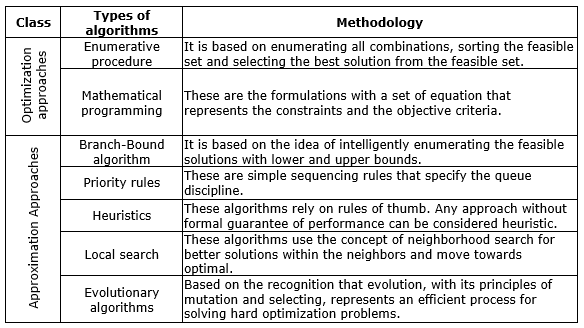
Few Pros and Cons that are faced by MOEAs while solving the optimization methods are:
-
The problem has multiple, possibly incommensurable, objectives.
-
The Computational time for each evaluation is in minutes or hours.
-
Parallelism is not encouraged.
-
The total number of evaluations is limited by financial, time, or resource constraints.
-
Noise is low since repeated evaluations yield very similar results.
-
The overall decline in cost accomplished is high.
SUMMARY AND CONCLUSIONS
Six population-based meta-heuristic algorithms have been reviewed; their working procedure is briefed, and the range of applications indicated. Since scheduling problems fall into the class of NP-complete problems, they are among the most difficult to formulate and solve. Operations Research analysts and engineers have been pursuing solutions to these problems for more than 35 years, with varying degrees of success. While they are difficult to solve, job shop scheduling problems are among the most important because they impact the ability of manufacturers to meet customer demands and make a profit. They also impact the ability of autonomous systems to optimize their operations, the deployment of intelligent systems, and the optimizations of communications systems. For this reason, operations research analysts and engineers will continue this pursuit well into the next century. This paper may not add to the existing body of literature, but reorganizes it; and, it also serves the effort of scoping further research in this direction.
REFERENCES
Cheng, S.-L.; Hwang, C. (2001), “Optimal Approximation of Linear Systems by a Differential Evolution Algorithm”, IEEE Transactions on Systems, Man, and Cybernetics-Part A: Systems and Humans, Vol.31, No. 6, 698–707.
Dorigo, M.; Gambardella, L. M. (1997), “Ant colonies for the travelling salesman problem”, Bio Systems, Vol. 43, No.2, pp.73-81.
Ghosha, T. et al. (2011) “Meta-heuristics in cellular manufacturing: A state-of-the-art review”, International Journal of Industrial Engineering Computations, Vol. 2, pp. 87–122.
Goldberg, E. D. (1989), Genetic algorithms in search optimization and machine learning, Addison Wesley Publishing Company Inc., New York, USA.
Ishibuchi, H. et al. (2003), “Balance between Genetic Search and Local Search in Memetic Algorithms for Multiobjective Permutation Flowshop Scheduling”, IEEE Transactions on Evolutionary Computation, Vol. 7, No. 2, pp. 204–33.
Jain, A. K. et al. (1999) “Data clustering: a review”, ACM Computer Survey, Vol. 31, No. 3, pp. 264–323.
Kalyanmoy, D. (2002), Optimization for Engineering Design, Prentice Hall, New Delhi, India.
Kennedy, J.; Ebehart, R. (1995), “Particle swarm optimization”, in: IEEE International Conference on Neural Networks, Perth, Australia, 1995, Vol.4, pp.1942-1948.
Kicinger, R. et al. (2005) "Evolutionary computation and structural design: a survey of the state of the art", Computers & Structures, Vol. 23-24, pp. 1943-78.
Lin, Y. -C., et al. (2004), “A Mixed-Coding Scheme of Evolutionary Algorithms to Solve Mixed-Integer Nonlinear Programming Problems”, Computers & Mathematics with Applications, Vol. 47, No. 8–9, pp. 1295–1307.
Mackworth, A.; Goebel, R. (1998), Computational Intelligence: A Logical Approach by David, Oxford University Press, Oxford, UK. ISBN 0-19-510270-3.
Onwubolu, G.; Davendra, D. (2006), “Scheduling flow shops using differential evolution algorithm”, European Journal of Operational Research, Vol. 171, No. 2, 674-92.
Osman, I. H.; Laporte, G. (1996) “Metaheuristics: a bibliography”, Operations Research, Vol. 6, pp. 513–623.
Price, K.; Storn, R. (1995), Differential Evolution—A Simple and Efficient Adaptive Scheme for Global Optimization Over Continuous Spaces, International Computer Science Institute of Berkeley, Berkeley, CA.
Qian, B. et al. (2008), “A hybrid differential evolution for permutation flow- shop scheduling”, International Journal of Advanced Manufacturing Technology, Vol. 38. No. 7–8, pp. 757–77.
Rao, R. V. et al. (2011), “Teaching-learning-based optimization: A novel method for constrained mechanical design optimization problems”, Computer-aided Design, Vol. 43, No. 3, 303-15.
Rao, R. V.; Kalyankar, V. D. (2010), “Parameter optimization of machining processes using a new optimization algorithm”, Materials and Manufacturing Processes, pp.978-85. DOI:10.1080/10426914.2011.602792.
Sajja, R.; Chalamalasetti, S. R. (2014), "A selective survey on multi-objective meta-heuristic methods for optimization of master production scheduling using evolutionary approaches.", International Journal of Advances in Applied Mathematics and Mechanics, Vol. 1, No. 3, pp. 109-20.
Schwefel, H. P. (1977), Numerische Optimierung von Computer-modellen mittels der Evolutionsstrategie, Birkhäuser Verlag, Basel, Swiss.
Tasgetiren, M. F. et al. (2007), “A discrete differential evolution algorithm for the no-wait flowshop problem with total flowtime criterion”, in: proceedings of the IEEE symposium on computational intelligence in scheduling, 2007, pp. 251–8.
Received: 30 Dec 2017
Approved: 10 May 2018
DOI: 10.14488/BJOPM.2018.v15.n1.a17
How to cite: Chaparala, A.; Sajja, R. (2018), “Optimization using evolutionary metaheuristic techniques: a brief review”, Brazilian Journal of Operations & Production Management, Vol. 15, No. 1, pp. 44-53, available from: https://bjopm.emnuvens.com.br/bjopm/article/view/412 (access year month day).