Using metaheuristic algorithms for solving a mixed model assembly line balancing problem considering express parallel line and learning effect
Masoud Rabbani
mrabani@ut.ac.ir
University of Tehran, Islamic Republic of Iran
Farahnaz Alipour
farahnaz.alipour@yahoo.com
University of Tehran, Islamic Republic of Iran
Hamed Farrokhi-Asl
hamed.farrokhi@alumni.ut.ac.ir
Iran University of Science & Technology, Islamic Republic of Iran
Neda Manavizadeh
n.manavi@khatam.ac.ir
KHATAM University, Islamic Republic of Iran
ABSTRACT
Mixed-model assembly line attracts many manufacturing centers' attentions, since it enables them to manufacture different models of one product in the same line. The present work proposes a new mathematical model to balancing mixed-model assembly two parallel lines, in which first one is a common line and the other is an express line due to more modern technology or operators with higher skills. Therefore, the cost of equipment and skilled labor in the express line is higher, and also, the learning effect on resource dependent task times and setup times is considered in the assemble-to-order environment. The aim of this study is to minimize the cycle time and the total operating cost and smoothness index by configuration of tasks in stations, according to their precedence diagrams. Also, assigning the assistants to some tasks in some stations and for some models is allowed. This problem is categorized as an NP-hard problem and for solving this multi-objective problem, non-dominated sorting genetic algorithm ІІ (NSGA-II) and multi-objective particle swarm optimization (MOPSO) are applied. Finally, for comparing the proposed methods some numerical examples are implemented and the result show that MOPSO outperforms NSGAII.
Keywords: Mixed-model assembly line; Balancing; Learning effect; Parallel line.
1. INTRODUCTION
In modern manufacturing systems, flexibility in product mix is a common problem to satisfy in a cost-effective manner when there are various customized demands. Moreover, because of the existing competitive environment for producers, the mixed-model assembly line attracts many manufacturing centers’ attentions that can manufacture different models of one product in same line. In assembly lines, balancing and sequencing are two main issues. Due to the increasing trend towards using the mixed model assembly line and the instability of market demand, these two issues have been taken into consideration by many researchers over the past two decades (Ramezanian and Ezzatpanah, 2015). Salveson (1955) published the first study in the assembly line balancing problem (ALBP). The main purpose of ALBP is to assign a limited set of tasks to workstations regarding the confirmation of precedence relations and to optimize some effectiveness measures, such as cycle time, number of workstations, line efficiency, or idle time (Erel and Sarin, 1998). Following the classification, Boysen et al. (2007) stated that ALBP can be classified into three groups, according to the number of models: single-model ALBP, whose only product is produced in the lines; multi-model ALBP different products are produced in batches; and mixed-model ALBP, varying models of one product are assembled on the same assembly processes. Reduction in investment production, risks of uncertainty environment and cost of equipment and also quick response to the different requirements are some of the advantages of the mixed model assembly lines (Erel, 1998, McMullen, 1997, Miltenburg, 2002).
For simplifying this problem, in simple assembly line balancing problems (SALBP), some assumptions are assumed. Until now these assumptions have been used in many studies (Baybars, 1986; Cakir et al., 2011; Michalos et al., 2010). In the sequence, these assumptions are discussed:
-
Considering mass production of the same model with a definite process
-
There is no substitute for processes.
-
Considering paced line with constant cycle time C.
-
Locating is linearly performed with m unilateral station and without any feeding lines or parallel lines.
-
The only limitation is prerequisite for the allocation of activities.
-
The duration time of activities is definitive.
-
An activity could not be divided in two separate stations.
-
All stations are equipped with the machinery and employees in the same way.
By changing variables, the different models of SALBP are obtained. In the following four main models for SALBP are described.
When the cycle time value is given and the aim of the problem is minimizing the number of station, the model of SALBP is type 1 (SALBP-1) and when the station number is given and the aim of the problem is to minimize the cycle time value, the problem is type 2 (SALBP-2).
When both of them are unknown variables and the aim of problem is to minimize the number of stations and cycle time simultaneously, considering the maximum efficiency, the model is converted to a simple assembly line, balancing problem, considering efficiency (SALBP-E).
Simple assembly line balancing feasibility problem (SALBP-F) is an NP-complete problem that, given both the number of station and the cycle time values, the feasibility of the problem is checked and a feasible solution is discovered. Thus, this method deals with the SALBP as a NP-hard problem (Rabbani et al., 2014). Therefore, by eliminating some simplified assumptions and adding up some constraint the SALBP addresses generalized assembly line balancing problem (GALBP) that is a more realistic model. In the following, the assumption of GALBP is discussed:
-
It is possible to produce more than one type of product.
-
A set of different alternative processes can be considered.
-
It is possible to plan the production line in such a way that it satisfies the amount of the target production in a certain planning horizon and this planning can be obtained by considering the cycle time average in computations.
-
Considering unidirectional flow line.
-
The sequence of activities follows the precedence limitations.
-
The 5 to 7 assumptions of SALBP are given up.
Mixed-model assembly line balancing (MMALB) is one of the GALBP problem that has greater flexibility than the single-model and the multi-model (Palau Requena, 2013). Generally, MMALBP-1, MMALBP-2 and MMALBP-E are three types of problems which are faced in the literature of MMALBP. The main purpose in MMALBP-1 (MMALBP-2) is to minimize the number of workstations (cycle time) for a given cycle time (number of workstations) and to utilize combined precedence diagram that converts all of the precedence diagrams into one diagram that has permissible orderings of the tasks for the M models (Gökċen and Erel, 1998). Considering flexible resource dependent operation times in assembling various models, MMALBP-2 seems to be more suitable for this problem.
Most of the research focused on the ‘operation’ time, which is the time of net value-adding processes, assumed that the task order has no effect on the inter-task times. However, in many real situations the task sequences remarkably affect the inter-task times (Scholl and Voß, 1997). Due to the importance of this issue in the system design, recently a few studies considered the sequence dependent setup times in a single model assembly line balancing problem (Scholl, 2008; Andres, 2008; Özcan, 2010). Nowadays, by increasing the variety requirement of customers and considering the mixed model assembly lines in production systems, the inter-task times attract more attention due to the main effect of switching time between different models on line performance that include setup change (Wilhelm, 1999). The remainder of this paper is structured as follows: a review of literature is described in section 2. A problem description and its mathematical formulation are given in Section 3. The solution procedures are presented in Section 4. Numerical examples are presented in Section 5. Finally, the conclusion of the article is provided in Section 6.
2. LITERATURE REVIEW
There are many researches on the ALBP in the literature (Becker and Scholl, 2006;Boysen et al., 2007; Boysen et al., 2008; Ghosh and Gagnon, 1989). Some well-known objective functions in ALBP are minimizing the number of workstations, minimizing the cycle time, maximizing the line efficiency (Boysen et al., 2007), maximizing workload smoothness (Nearchou, 2008), minimizing the smoothness index presented by Ponnambalam et al. (2000), and minimizing the total cost (Jayaswal and Agarwal, 2014; Tiacci, 2015).
Due to many advantages, such as ease of balance workload between stations, increased reliability, more flexibility in scheduling, worker satisfaction, a parallel arrangement of lines that provides further improvements in terms of flexibility, and sensitivity to fail was used. Therefore, the use of parallel mixed model assembly lines is improving system performance and increasing productivity (Süer, 1998). Süer (1998) was the first author to consider parallel assembly lines very limited, as well as studies on single model parallel assembly lines balancing have reported the same, as in the case of Benzer et al. (2007), Scholl and Boysen (2009), and Gökçen et al. (2006), and he defined a problem in designing parallel assembly lines when the number of productions is too high and there are more workers required and the objective is to find out the number of assembly lines that minimizes total manpower.
Reducing the number of workstations, and subsequently, reducing the idle time, and reducing the cycle time and achieving high production rates are the other advantages that could be achieved by using parallel assembly lines (Bukchin and Rubinovitz, 2003, BARD, 1989).
Gökçen et al. (2006) examined the balancing of the parallel assembly lines. Scholl and Boysen (2009) proposed a model for designing parallel assembly lines with split workplaces and they indicated that increased productivity can be combined with the adjacent stations and also the objective function is to minimize the work space and the number of operators. Ozbakir et al. (2011) presented one of the first attempts in terms of modeling and solving the parallel assembly line balancing problem wherein they used swarm-intelligence-based metaheuristics. Rabbani et al. (2014) used genetic algorithm (GA) to solve MMALB, considering express parallel line that works faster and produces similar mixed products, and also they considered different alternatives for selling products. Kucukkoc and Zhang (2015) developed a heuristic algorithm for maximizing resource utilization in parallel U-shaped assembly line balancing problem.
Boysen et al. (2008) defined the mixed model assembly line as a varied sequential model of a standard product. Models may vary in terms of color, size, materials, equipment, precedence, relationships of tasks, and task durations. There are several common tasks with the same priority relationship between different models on a mixed model assembly line. This is used by Thomopoulos (1970) to considerably reduce the number of variables and constraints in the model.
Matanachai & Yano (2001) offered a new approach to balancing mixed model assembly lines and they focused on the allocation of tasks to workstations by creating a daily sequence of customer orders. They introduced a new goal for the mixed model assembly line balancing to achieve a stable workload in the short term with a heuristic solution. In addition, they have assumed that the number of stations and the cycle time is predetermined. Simaria & Vilarinho (2004) stated that, nowadays, the market is moving towards products with more diversity. Thus, the mixed model assembly line is preferable to the traditional single assembly line. Therefore, they provided a mathematical programming model and an iterative process based on genetic algorithm to the problem of mixed model assembly line balancing with parallel workstations and the goal of maximizing the rate of production of assembly line with a predetermined number of workstations.
Hamta et al. (2011) used lower and upper bounds for task time and called this type flexible operation time. The paper aimed to minimize the cycle time and minimize machine total costs. Nima Hamta (2013) considered flexible operation times, sequence-dependent setup times, and learning effects in a hybrid particle swarm optimization (PSO) algorithm, minimizing the cycle time, minimizing the total equipment cost, and minimizing the smoothness index. Assigning operators and activities to the stations is an important issue for balancing the assembly lines. Therefore, a model for maximizing production rate and balancing workloads among operators on the assembly line has been created by Purnomo and Wee (2014).
Ramezanian and Ezzatpanah (2015) proposed a model for worker assignment problem. They assign workers to workstations with considered operating costs and their abilities to minimize cycle time and all the cost that are related to workers. They used Imperialist competitive algorithm (ICA) for tackling the problem, and the obtained results are compared with GA.
Many studies have assumed that a task needs a fix number of operators and machines; however, in real situations, for reducing the time of tasks, extra resources can be used. For this issue, a simulated annealing (SA) algorithm for solving a U-shaped assembly line balancing with resource dependent task times was presented by Jayaswal and Agarwal (2014). The best research on resource dependent u-shaped assembly line balancing (RDULB), which assigns tasks to workstations and minimizes total cost simultaneously, was presented by Yakup Kara (2011).
Reducing the setup times to zero is one of the main issues in lean manufacturing systems and makes to order environment. Zero setup time means there is no justification for the use of large stacks and it is better to choose producing batches one by one. Also, one of the important causes for reduction in efficiency is the setup time. Thus, considering an optimum sequencing for the tasks is necessary. Scholl et al. (2013) proposed a heuristic algorithm for minimizing the number of workstations with consideration of sequence-dependent setup time for a single model assembly line balancing problem. Moreover, Nazarian (2010) and Kara (2007) considered set up time in their studies for mixed model assembly lines and showed the impact of sequence dependent setup times to obtain the best sequence of tasks.
Repeating an activity over the time increases the speed of operators and, considering the learning effect in ALBP, it creates conditions with dynamic task times. Biskup (1992) was the first author that analyzed learning effect in single-machine scheduling problems and the objective functions are minimize the deviation from a common due date and the sum of flowtimes. Toksari, İşleyen (2008) and Nima Hamta (2013) used a heuristic algorithm and they utilized Biskup’s approach for considering learning effect into single model assembly line balancing problems. Zhao et al. (2015) proposed a GA that considers mental workload in mixed-model assembly line to maximize the production efficiency in straight line and the Weibull distribution was used to describe the relationship between working performance and mental workload.
Manavizadeh et al. (2013) presented a model for reducing the number of stations and maximizing the weighted efficiency in U-shaped and mixed-model assembly line balancing problem using SA. Özcan et al. (2011) developed a GA to solve the mixed-model U-line balancing and sequencing problem when considering stochastic task times. Table 1 summarizes some relevant studies in the literature and highlights gaps between studies.
The present work proposes a new mathematical model to minimize the cycle time and the total operating cost related to resource dependent task times and smoothness index with considering simultaneously flexible operation times, sequence-dependent setup times and learning effect in assemble-to-order environment for two parallel lines, in which the first one is a common line and the other, due to more modern technology or operators with higher skills, is an express line. Therefore, the cost of equipment and skilled labor in the express line is higher and, as a result, the price and product quality is higher than the common line. However, in order to respond more quickly to customers' requirements, as well as to have better control over costs and selling price, it is allowed to consider these two lines together and in parallel shape.
3. PROBLEM DESCRIPTION
In this paper, a multi-objective model for solving the MMALB problem is proposed when considering express parallel line, resource dependent task times, flexible operation times, sequence-dependent setup times and learning effect in assemble-to-order environment. In order to describe the problem, the basic assumptions must be introduced. Moreover, a schematic figure of the proposed problem is shown in Figure 1.
Figure 1. Distribution of entering materials
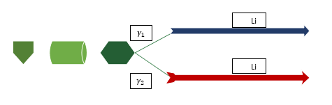
Source: The author(s)’ own
3.1 Assumption
- The models are homogeneous and all parts of the models are prepared for utilization in the assembly line.
- Some kinds of customers are interested to pay a higher cost for reducing delivery time and this higher payment allows the manufacturer to consider particular condition in this manufacturing opportunity.
- It is considered an express parallel line with higher performance operator and higher speed (and quality) that is equipped by high-level machinery beside the common (main) assembly line. Thus, the lead time of express line is reduced.
- The workers are trained to perform any operation in each line. Moreover, some tasks can be processed with additional resources (equipment or assistant).
- We have lower bound Lti and upper bound Uti of each operation task time.
- Task durations depend on the type of resource (equipment type or assistant) used and using additional resources decreases the task duration.
- GALBP is studied using the learning curve described by Biskup (1999), in which the learning effect is considered on the operation time of task i assigned to position r by the following formulation:

where α (=log2s ≤ 0) is the learning effect and s denotes the learning rate
- The setup times are known and deterministic.
- Regular operators and assistants can move between crossover workstations. The sufficient number of regular operators is available to operate the workstations, but other resources (equipment and assistants) are limited.
3.2. Mathematical model
The multi-objective GALBP, considering express parallel line, resource dependent task times, flexible operation times and learning effect in assemble-to-order environment, can be formulated as the following mixed integer nonlinear programming model. Furthermore, in Figure 1 the distribution of materials that enter to the lines is described.
3.2.1 Mathematical formulation

The concept of total cost (TC) is utilized for reducing number of variables in the second objective.
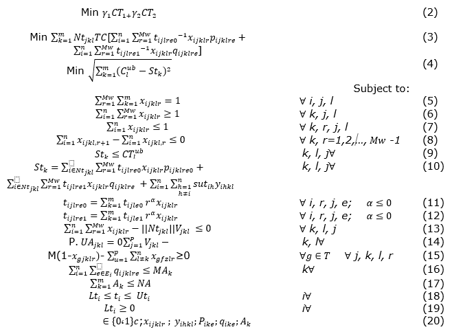
Equations (2)-(4) are the objective functions. While objective function (2) minimizes the average of cycle time for two lines, equation (3) minimizes the total cost and relation (4) minimizes the smoothness index. Constraints (5) implies that each task of each model can be assigned in only one sequence position in only one workstation in each line. Constraints (6) and (7) ensure that each workstation is assigned by, at least, one task and each sequence position inside each workstation will have at most one assigned task. Constraints (8) state that, for assigning tasks in sequencing each workstation, the ascending order of positions should be noticed. (9) is the cycle time constraints that states that the sum of operation times when considering learning effect and setup times in each workstation should not exceed the Upper bound cycle time of line l. Constraint (10) computes the time of workstation k. Constraints (11) and (12) determine the operation time of task i when considering the effect of learning if task i assigned to position r, where α is a learning index.
Constraints (13) and (14) guarantee the utilization of all the stations for all models and, if a station is not utilized for one model, it should not be used for other models. These constraints are presented by Gökċen and Erel (1998). Constraints (15) are used to assign common tasks of models to the same station on each line. Constraints (16) state that an assistant cannot operate a task at a workstation unless one is assigned to that workstation. Constraints (17) are the assistant availability constraints. Constraints (18) guarantee that operation times must be between given lower and upper bounds. Constraints (19) denote the state of the lower bounds of operation times. Constraint (20) considers binary variables.
4. METHODOLOGY
Two solution algorithms have been applied to detect rational Pareto solutions. This section examines the details of these two proposed methods for solving a mathematical model. The first method is non-dominated sorting genetic algorithm (NSGA-II) and another is multi-objective particle swarm optimization algorithm (MOPSO). These two methods have been used in many studies and they are well-known as an efficient method among researchers (Ghodratnama et al., 2015).
4.1. Chromosome representation
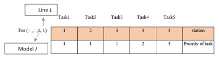
In this study, for resolving the problem, the number of components in each chromosome is equal to a given number of models and assembly lines. It should be noted that each chromosome associates with one solution in solutions space. Each component has two rows and the length of matrix is defined by the number of tasks. The first row represents the assignment of tasks to station and the second row shows the priority of tasks. A sample matrix for the first model, first line, and five tasks are shown in Figure 2. In this problem, if we have J model then we should have 2J matrices in each solution because of the existence of two parallel lines and each matrix consists of two rows. For example, this matrix states that the tasks number 1 and 2 are done by first and second stations, respectively, and task 3, 4 and 5 are done by the third station, respectively.
Figure 2. Chromosome representation
Source: The author(s)’ own
4.2. NSGA-II algorithm
Srinivas & Deb (1994) proposed NSGA-II for solving multi-objective problem for the first time. The main difference between the algorithm of this method and GA is the way of selecting the members of a new population. NSGA-II uses the fast non-dominated sorting approach to rank the whole population and, when it is not possible to compare ranks, it uses a crowding distance for comparing and selecting the population fronts. In the following subsections, the steps of NSGA-II algorithm are presented in detail.
4.2.1. Generating the initial population
Generating the initial population (P0) in size of N is the first step of this algorithm and all individuals of P0 employed non-dominated sorting and crowding distance procedure for ranking the members of the population.
In this study, the assignment of stations to the tasks for each line and each model can be specified by the following construction algorithm to initialize the population. The steps of construction algorithm to generate the initial population are as follows:
Step 1: Assign station 1 to the task 1.
Step 2: Input the immediate follower of assigned tasks to command list.
Step 3: Assign station 1 to the task with more priority and check the Ei and Li constraints for feasibility. If these constraints are not feasible, assign the next priority.
Step 4: Control the time of the stations that is not exceeded by the task duration time that is assigned in them. If it is exceeded, open the new station and go back to step 2 else; if it is less, go back to step 2 and, according to the task times and their precedence relations, if possible, assign the other task in the same station.
Step 5: Make iteration to assign all tasks to stations.
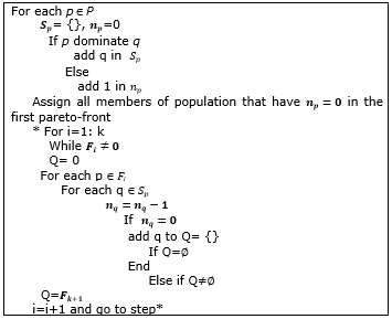
4.2.2. Rank calculation for solutions
When none of objective functions dominate each other and we could not choose the best solution, the non-dominated is ranked between the solutions done and is compared to any rate in one of the objective functions that is better than the others. According to Deb et al. (2002), the non-dominated sorting algorithm is described in Figure 3.
Figure 3. Non-dominated sorting algorithm
Source: The author(s)’ own
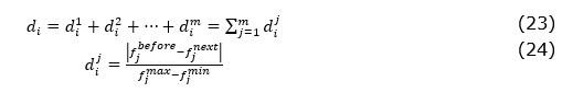
4.2.3. Crowding distance
According to Deb et al. (2002), an important attribute of NSGA-II that differs this algorithm from others is crowding distance. It determines the relation of individuals with their neighbor in terms of their distance from each other. The summaries of finding crowding distance are as follow: f_i is an objective function and d_i is distance.
4.2.4. Parent selection
Binary-tournament selection is applied to select parents. First, two random solutions from the population should be specified. If they have different rank, the solution with lower rank will be chosen; or else, the solution with higher crowding distance will be selected.
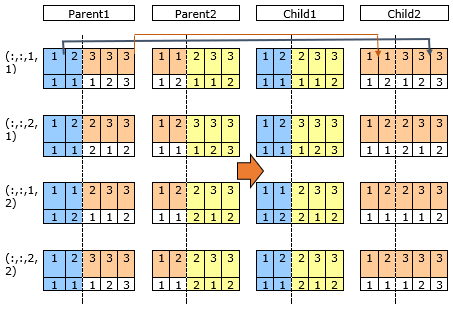
4.2.5. Crossover
After selecting parents, the crossover operator is used to create two offsprings by combining the two parents and then these two children are added to the offspring population. This operator firstly produces an integer random number between one and the length of chromosomes. Then the right part of chromosomes of the first parent is transferred to the right side of the chromosomes of the second parent or the left side of the chromosome of the second parent is transferred to the left side of the chromosome of the first parent. The crossover operator is shown in Figure 4.
Figure 4. Crossover procedure
Source: The author(s)’ own
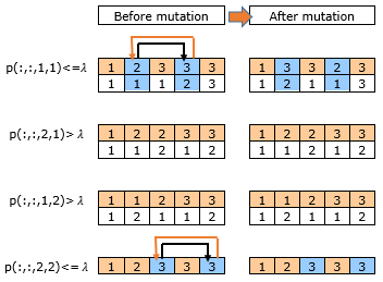
4.2.6. Mutation
Another operator is the mutation operator, which generates another possible solution. As it is shown in Figure 5, in this algorithm, after developing a new individual, each gene with the mutation probability will be transformed. When the mutation occurs, maybe a gene is removed from the set of genes or it may be the gene that has ever existed in the population added to this set. The mutation of a gene means that the gene changes and, depending on the type of coding, mutations are used in different ways. In this study, for each model (j) and line (l) in each chromosome matrix whose probability is lower than λ, two random numbers are generated for task (i) and swapping them with each other.
At last, after generating the children by crossover and mutation, it is necessary to control the feasibility of constraints for each chromosome (as earlier or latest time of station constrains or precedence constrains of tasks) and repair them.
Figure 5. Mutation procedure
Source: The author(s)’ own
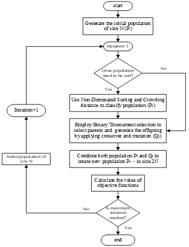
4.2.7. Generating New Population
By combining the population Pt and children Qt, a combined population, (Rt), in size 2N will be generated (i.e., (Rt) = {(Pt) ∪(Qt)}).
The procedure is continued with a non-dominated sorting of combined population to obtain the Pareto fronts and estimation of crowded distance of solutions in each front. The next parent population ((Pt)+1), in size N, is formed by selecting the best individuals, according to their rank and crowded distance. The algorithm is terminated after performing a constant number of generations. The algorithm of NSGA-II is described in Figure 6.
Figure 6. Flowchart of NSGA-II algorithm
Source: The author(s)’ own
4.3. Multi-objective particle swarm optimization
Particle swarm optimization is one of the newest evolutionary optimization techniques that was developed by Eberhart and Kennedy (1995) for the first time. The basic idea of PSO derived from the social behavior of a group of birds. Since the use of this algorithm requires only a series of elementary arithmetic operators, the implementation of this algorithm is simple and economical in terms of costs.
Multi-objective particle swarm optimization algorithm (MOPSO) was introduced by Coello et al. (2004). It is an extension of PSO algorithm and it is used for solving multi-objective problems. Because of the existence of multi objective in MOPSO, a concept called archive or repository is added in MOPSO compared to PSO, whose member of the repository represents Pareto Front and its particles are non-dominated.
The most important and essential step for each particle is choosing the best answer from global best (Gbest) answer and the best personal recollection. Thus, in MOPSO against PSO, there is set of non-dominated particles; therefore, one member of repository is chosen as a leader and the new velocity and position of each particle is computed by the employing equation 25 and 26 that is presented below:
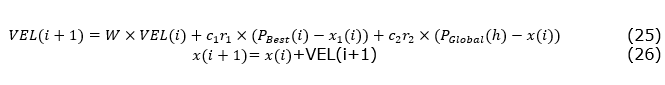
Where w is called inertia weight that is responsible for controlling the impact of the past velocity of each particle on the current one. c1 and c2 are called cognitive and social positive parameters, respectively. PBest(i) is the best memory of particle i and PGlobal(h) is the value of leader member in hyper cubes h that has more particles than other hyper cubes.
For comparing the best vector of personal recollection, use the following syntax:
- If the new position dominates the best memory, then the new location is the best memory.
- If the new position is dominated by the best memory, then do nothing.
- If none of them beat each other, consider one of the best positions as leader.
In the following, the algorithm of MOPSO is described in Figure 7.
Figure 7. Flowchart of MOPSO algorithm
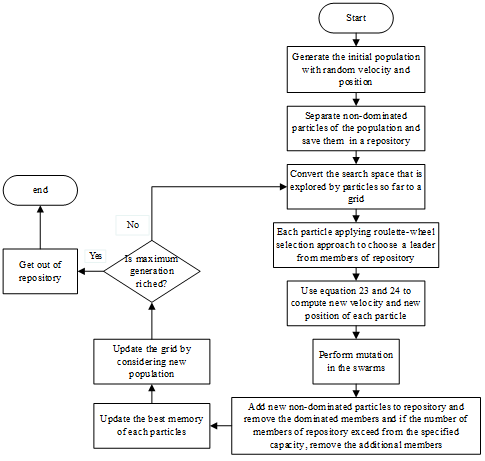
Source: The author(s)’ own
5. Experimental results
In this section, the proposed NSGA-II and MOPSO are compared with each other and the results are analyzed. MATLAB R2012a on Intel CORE i5 2.40 GHz personal computer with 4 GB RAM is used for coding the algorithms.
5.1. Parameters tuning
For obtaining the tuned value of each parameter of algorithms, the Taguchi design of experiment on MINITAB 17 is applied, based on the number of Pareto solution.
For optimizing the proposed algorithm parameters, some designed set of experiments prefer the Taguchi method (2005) that has considerable effect on improving the quality of the algorithm. Actually, this method assigns a set of experiments with different values of the parameters to minimize the effect of some causes that could affect the results by producing variation in them.
In the first phase, this method was concerned with the identification of the parameters that could affect the results and a certain level for each value of the parameter is assigned to them. For example, in the NSGA-II algorithm, the number of population, maximum number of iteration, crossover and mutation parameters and in the MOPSO algorithm, the number of population, maximum number of iteration, number of repository, cognitive and social positive parameters, and inertia weight might influence the results.
Figure 8-9 and Table 2 indicate the result of the analysis of Taguchi Design and the tuned value of each parameter with their different levels for the proposed NSGA-II and MOPSO algorithms. In this study, three levels for each parameter are considered and, for each level, five numbers of experiments are performed. The current set of experiments is used to test 25 experiments containing three levels and five different parameters.
Figure 8. The result of Taguchi design for the NSGA-II algorithm
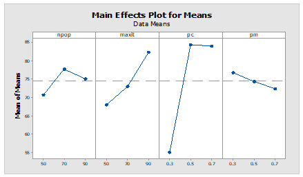
Source: The author(s)’ own
Figure 9. The result of Taguchi design for the MOPSO algorithm
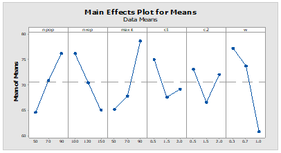
Source: The author(s)’ own
5.2. Test problems
Two section including small and large problems are considered to implement the experimental results. In this paper a set of eight MMALBP instances, including five small sized and three large sized problems, are considered to calculate the objectives by using the NSGA-II and MOPSO algorithms. In this section, the forth example from small instances and the second example from large size instances are explained. The information of these two problems involving precedence diagrams, task dependent setup times, cost of equipment in each line, cost of workstation and assistant, and the probability of entering to each line are in appendix, and the information about their task times and other instances are available in https://goo.gl/Yu1nIE.
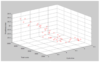
The information of parameters that is used in examples 1 and 2 is shown in Table 3 and the Pareto result of two algorithms for both examples are shown in Table 4-5 and Table 7-8. Moreover, in Figure 10-13 the Pareto front of NSGA-II and MOPSO for both examples are shown. The reply of solutions 15 and 18 of NSGA-II for both examples are shown in Table 6 and Table 9, respectively. For example, the result in Table 6 indicates that, in line 1 and station 1 for task 1, one assistant should be assigned for model 1.
Figure 10. The Pareto front of NSGA-II for example 1
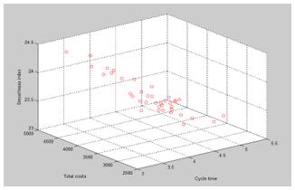
Source: The author(s)’ own
Figure 11. The Pareto front of MOPSO for example 1
Source: The author(s)’ own
Figure 12. The Pareto front of NSGA-II for example 2
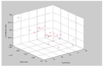
Source: The author(s)’ own
Figure 13. The Pareto front of MOPSO for example 2
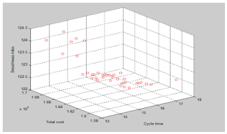
Source: The author(s)’ own
5.3. Comparison metrics
It is necessary to evaluate the quality of the generated Pareto fronts’ solutions for comparing two algorithms. There are different measures for comparing different algorithms. In this paper, four popular performances’ metrics, including number of Pareto, diversity, spacing, and mean ideal distance (MID) is considered to indicate the efficient algorithm between NSGA-II and MOPSO for this problem. In the following, these four measures are explained:
• Number of Pareto front: by using this measure we could recognize the ability of algorithms to discover an efficient solution.
• Diversity: it indicates the extension of non-dominated solutions and it computes as follow:
Where  are the non-dominated solutions,
  is the Euclidean distance between them, and n is the number of non-dominated solutions (Knowles and Corne, 2002).
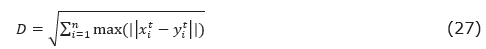
- Spacing: this metric measures the distribution of the Pareto front solutions by computing the distance variance of the neighboring solution in the Pareto front.
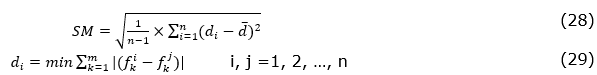
Where m is the number of objectives, n is the number of non-dominated solutions, and  is the mean value of all di. The less SM for each Pareto front solution means the more efficient solution.
- Mean ideal distance: this metric indicates the sum of the distance of solutions from the ideal point of Pareto that computed as follows:
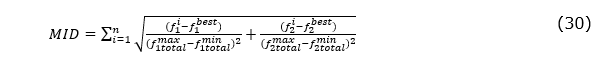
Where  is the maximum value of the objective function, and
  are the ideal points. Smaller MID value is more preferred.
Table 10 summarizes the result of each measure for five small and three large size instances. According to this table, generally, the performance of MOPSO, such as more number of Pareto solution and diversity, is better in comparison with NSGA-II. The value for mean ideal distance and spacing in most instances in MOPSO is smaller than NSGA-II.
CONCLUSION
In order to respond quickly to customer demands by considering affordable prices and their satisfaction, production and assembly systems need to have a schedule and a plan for balancing the lines. Thus, they can reduce costs and increase quality and efficiency, and also, by the effective cost, they can respond to all requests. In this study, the NSGA II and MOPSO algorithms were applied to solve a mathematical model of balancing mixed-model assembly lines when considering an express parallel line to respond the orders quickly and the learning effect on resource dependent task times and setup times in assemble-to-order environment. The aim of this study was to minimize the cycle time, the total operating cost, and the smoothness index simultaneously, by configuring tasks in stations, according to their precedence diagrams and also to assign the assistants to some tasks in some stations and for some models that optimize the objectives. The costs that are considered in this objective are costs of equipment on each line, cost of workstation, and cost of assigning an assistant to tasks. Therefore, it is rational to assign an assistant to some tasks to accelerate the implementation operations and minimize the cycle time.
For recognizing the efficiency of NSGA-II and MOPSO, eight numerical examples in small and large size problems were applied and the result is indicated in the Pareto solution of two examples in the context. Finally, we concluded that gaining the best position of tasks for each model, considering minimizing these three objectives, is possible as well as the result of comparing these two algorithms represent the highest number of Pareto front solution and diversity in MOPSO, compared with NSGA-II in all instances and better performance of MOPSO according to the spacing and MID metrics in the majority of instances.
The result of such studies could help the managers to increase their customers and the speed of response of their variable demand and minimize the total cost of systems simultaneously. For future research, using this constraint in parallel with the U-shaped assembly line or other configuration of lines, also considering uncertainty in task times and equipment reliability, could be effective.
REFERENCES
Bard, J. F. (1989), “Assembly line balancing with parallel workstations and dead time”, The International Journal of Production Research, Vol. 27, pp. 1005-18.
Baybars, I. (1986), “A survey of exact algorithms for the simple assembly line balancing problem”, Management Science, Vol. 32, 909-932.
Becker, C.; Scholl, A. (2006), “A survey on problems and methods in generalized assembly line balancing”, European Journal Of Operational Research, Vol.168, pp. 694-715.
Benzer, R. et al. (2007), “A network model for parallel line balancing problem”, Mathematical Problems in Engineering.
Biskup, D. (1999), “Single-machine scheduling with learning considerations”, European Journal of Operational Research, Vol. 115, pp. 173-8.
Boysen, N. et al. (2007), “A classification of assembly line balancing problems”, European Journal of Operational Research, Vol. 183, pp. 674-93.
Boysen, N. et al. (2008), “Assembly line balancing: Which model to use when?”, International Journal of Production Economics, Vol. 111, pp. 509-28.
Bukchin, J.; Rubinovitz, J. (2003), “A weighted approach for assembly line design with station paralleling and equipment selection”, IIE Transactions, Vol. 35, pp. 73-85.
Cakir, B. et al. (2011), “Multi-objective optimization of a stochastic assembly line balancing: A hybrid simulated annealing algorithm”, Computers & Industrial Engineering, Vol. 60, pp. 376-84.
Coello, C. A. C. et al. (2004), “Handling multiple objectives with particle swarm optimization”, Evolutionary Computation, IEEE Transactions on, Vol. 8, pp. 256-79.
Deb, K. et al. (2002), “A fast and elitist multiobjective genetic algorithm: NSGA-II.”, Evolutionary Computation, IEEE Transactions on, Vol. 6, pp. 182-97.
Eberhart, R. C.; Kennedy, J. (1995), “A new optimizer using particle swarm theory. Proceedings of the sixth international symposium on micro machine and human science”, in: Sixth International Symposium onMicro Machine and Human Science, New York, NY, 1995, pp. 39-43.
Erel, E.; Sarin, S. C. (1998), “A survey of the assembly line balancing procedures”, Production Planning & Control, Vol. 9, pp. 414-34.
Ghodratnama, A. et al. (2015), “Solving a new multi-objective multi-route flexible flow line problem by multi-objective particle swarm optimization and NSGA-II”, Journal of Manufacturing Systems, Vol. 36, pp. 189-202.
Ghosh, S.; Gagnon, R. J. (1989), “A comprehensive literature review and analysis of the design, balancing and scheduling of assembly systems”, The International Journal of Production Research, Vol. 27, pp. 637-70.
Gökçen, H., Ağpak, K.; Benzer, R. (2006), “Balancing of parallel assembly lines”, International Journal of Production Economics, Vol. 103, pp. 600-9.
Gökċen, H.; Erel, E. (1998), “Binary integer formulation for mixed-model assembly line balancing problem”, Computers & Industrial Engineering, Vol. 34, pp. 451-61.
Hamta, N. et al. (2011), “Bi-criteria assembly line balancing by considering flexible operation times”, Applied Mathematical Modelling, Vol. 35, pp. 5592-608.
Hamta, N. et al. (2013), “A hybrid PSO algorithm for a multi-objective assembly line balancing problem with flexible operation times, sequence-dependent setup times and learning effect”, International Journal of Production Economics, Vol. 141, pp. 99–111.
Jayaswal, S.; Agarwal, P. (2014), “Balancing U-shaped assembly lines with resource dependent task times: A Simulated Annealing approach”, Journal of Manufacturing Systems, Vol. 33, pp. 522-34.
Knowles, J.; Corne, D. (2002), “On metrics for comparing nondominated sets. Evolutionary Computation, 2002. CEC'02”, proceedings of the 2002 Congress on, 2002, IEEE, pp.711-16.
Kucukkoc, I.; Zhang, D. Z. (2015), “Balancing of parallel U-shaped assembly lines”, Computers & Operations Research, Vol. 64, pp. 233-44.
Manavizadeh, N. et al. (2013), “A Simulated Annealing algorithm for a mixed model assembly U-line balancing type-I problem considering human efficiency and Just-In-Time approach”, Computers & Industrial Engineering, Vol. 64, pp. 669-85.
Michalos, G. et al. (2010), “Dynamic job rotation for workload balancing in human based assembly systems”, CIRP Journal of Manufacturing Science and Technology, Vol.2, pp. 153-60.
Nearchou, A. C. (2008), “Multi-objective balancing of assembly lines by population heuristics”, International Journal of Production Research, Vol. 46, pp. 2275-97.
Ozbakir, L. et al. (2011), “Multiple-colony ant algorithm for parallel assembly line balancing problem”, Applied Soft Computing, Vol. 11, pp. 3186-98.
Özcan, U. et al. (2011), “A genetic algorithm for the stochastic mixed-model U-line balancing and sequencing problem”, International Journal of Production Research, Vol. 49, pp. 1605-26.
Ponnambalam, S. et al. (2000), “A multi-objective genetic algorithm for solving assembly line balancing problem”, The International Journal of Advanced Manufacturing Technology, Vol. 16, pp. 341-52.
Purnomo, H. D.; Wee, H. M. (2014), “Maximizing production rate and workload balancing in a two-sided assembly line using Harmony Search”, Computers & Industrial Engineering, Vol. 76, pp. 222-30.
Rabbani, M. et al. (2014), “Mixed-model assembly line balancing in assemble-to-order environment with considering express parallel line: problem definition and solution procedure”, International Journal of Computer Integrated Manufacturing, Vol. 27, pp. 690-706.
Ramezanian, R. & Ezzatpanah, A. (2015), “Modeling and solving multi-objective mixed-model assembly line balancing and worker assignment problem”, Computers & Industrial Engineering, Vol. 87, pp. 74-80.
Requena, O. P. (2013), The Time and Space Assembly Line Balancing Problem: modelling two new space features, Master thesis in Industrial Engineering, Universiteit Gent, Gent, Belgium.
Salveson, M. E. (1955), “The assembly line balancing problem”, Journal of industrial engineering, Vol. 6, pp. 18-25.
Scholl, A. et al. (2013), “The assembly line balancing and scheduling problem with sequence-dependent setup times: problem extension, model formulation and efficient heuristics”, OR Spectrum, pp. 1-30.
Scholl, A.; Boysen, N. (2009), “Designing parallel assembly lines with split workplaces: Model and optimization procedure”, International Journal of Production Economics, Vol. 119, pp. 90-100.
Scholl, A.; Voß, S. (1997), “Simple assembly line balancing—Heuristic approaches”, Journal of Heuristics, Vol. 2, pp. 217-44.
Süer, G. A. (1998), “Designing parallel assembly lines”, Computers & industrial Engineering, Vol. 35, pp. 467-70.
Thomopoulos, N. T. (1970), “Mixed model line balancing with smoothed station assignments”, Management Science, Vol. 16, pp. 593-603.
Tiacci, L. (2015), “Simultaneous balancing and buffer allocation decisions for the design of mixed-model assembly lines with parallel workstations and stochastic task times”, International Journal of Production Economics, Vol. 162, pp. 201–15.
Wilhelm, W. E. (1999), “A column-generation approach for the assembly system design problem with tool changes”, International Journal of Flexible Manufacturing Systems, Vol. 11, pp. 177-205.
Yakup Kara , C. Ö. et al. (2011), “Balancing straight and U-shaped assembly lines with resource dependent task times”, International Journal of Production Research, Vol. 49, pp. 6387–405.
Zhao, X. et al. (2016), “A genetic algorithm for the multi-objective optimization of mixed-model assembly line based on the mental workload”, Engineering Applications of Artificial Intelligence, Vol. 47, pp. 140-46.
Appendix
Figure 14. Precedence diagram of example 1
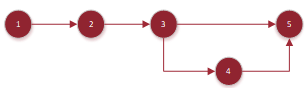
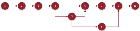
Figure 15. Precedence diagram of example 2
Received: 12 Jan 2017
Approved: 08 May 2018
DOI: 10.14488/BJOPM.2018.v15.n2.a8
How to cite: Rabbani, M., Alipour, F., Farrokhi-Asl, H. et al. (2018), “Using metaheuristic algorithms for solving a mixed model assembly line balancing problem considering express parallel line and learning effect”, Brazilian Journal of Operations & Production Management, Vol. 15, No. 2, pp. 254-269, available from: https://bjopm.emnuvens.com.br/bjopm/article/view/414 (access year month day).