A manufacturing bottleneck case study trough the theory of constraints and computational simulation of the proposed bottleneck solution
Gustavo Lemes Leite Barbosa
pregustavomium@gmail.com
University of Campinas – UNICAMP, Campinas, São Paulo, Brazil.
Robert Eduardo Cooper Ordoñez
cooper@fem.unicamp.br
University of Campinas – UNICAMP, Campinas, São Paulo, Brazil.
Rosley Anholon
rosley@fem.unicamp.br
University of Campinas – UNICAMP, Campinas, São Paulo, Brazil.
Mauricio Andrés Sanchez
mascphd@icloud.com
TecnipFMC - MPSG, Houston, Texas, United States of America.
Abstract
In 2016, the Brazilian pet industry had revenue of R$ 18.9 billion and ranked third place worldwide. Thus, it is a sector that is always looking for enhancements in its productivity levels. Based on the previous statements, a case study was conducted in a selected company of the pet care business, with the goal to augment its monthly revenue, identify the bottleneck that impedes reaching this goal, and proposed solutions to bring the production and loading fluxes of merchandise to its optimal state, making the company’s revenue also optimal. The classical tools of the theory of constraints were used in this analysis. The first step was to obtain the undesirable effects of the process to define the bottleneck. After that, some injections were proposed as solutions to eliminate the undesirable effects and bring the production and loading model of the company to its full state. Finally, by means of a computational tool, the current situation of the company (with the bottleneck), and the situation in a virtual state (without the bottleneck) were simulated and compared, showing the potential of the found solution.
Keywords: Theory of constraints; Computational simulation; Discrete event simulation; Case study.
1 Introduction
According to the Brazilian pet industry product association (ABINPET), Brazil has the second largest population of dogs, cats, and ornamental and singing birds in the world; the country is ranked in the third position when it comes to revenue in this same market. The productive chain related to the pet sector in Brazil had revenue of R$18.9 billion (US$ 5.7 billion) in 2016, of which 67.5% correspond to animal food (ABINPET, 2016).
Because of its size, the Brazilian pet market has several companies, represented by international and national capital acting as players in its productive chain with goals of not only augmenting their market share but also making their production and distribution processes more efficient and profitable.
In this context, one company of the sector was selected to be study-object of a case study involving the application of the Theory of Constraints (TOC). This study aimed to find out solutions to problems that did not allow the production and distribution fluxes to be optimal at the selected company. After the TOC methodology was applied, simulations were made to test its outputs.
Before making any sort of study regarding the TOC, it is indispensable that a goal is established for a systematic application of the method associated with the theory. In this case study, the established goal was to increase the company’s revenue at the end of each month, giving the fact that the quantity of orders made by the company clients increases tremendously and the challenge of loading the loads associated with these orders becomes much bigger. In these periods, the loading process faces two major problems; first, the availability of the products when a client’s truck to be loaded arrives at the company’s distribution center; and second, the agility of the loading process.
This work aims to register the data collected at the company where this case study has been applied, to present the results obtained by the application of the TOC’s method and finally to present a computational simulation of the obtained results to evaluate their effectiveness.
2 Theoretical framework
In this case-study, a goal has been set: increasing the company’s revenue at the end of each month. The TOC theory was selected to find the main constraint that did not allow attaining the goal. In the TOC thinking, the activities planning, execution and control should be done through the Constraint Management paradigm by means of a Continuous Improvement Methodology.
Considering a core goal and one identified constraint impeding this goal achievement, the objective of the methodology of the theory of constraints is to act on the constraint that is impeding the system to achieve this core goal (Santos et al., 2010).
The Israeli physicist Eliyahu Goldratt in the book “The Goal” has first proposed the Theory of Constraints in 1984. In the book, he has elucidated the theory that was conceived to bring improvements to the manufacturing environment, simplifying the amount of entry variables and using a standard method.
In this book, the authors write about five steps, known as the focusing steps that must be applied to implement the TOC methodology. They are: (1) locate the bottleneck(s); (2) create strategy on how to bring the bottleneck(s) efficiency to an optimal state; (3) adapt the other resources (i.e the non-bottleneck resources) to the proposed strategy on step two, making them collaborate with the proposed strategy; (4) invest in additions to the system so the bottleneck would have more capacity; and (5) to prevent the system from going back to an inertial state the process must restart in a cyclic fashion (Goldratt et Cox, 2004).
Through this algorithm and with the application of the tools related to the TOC, a systematic approach can be applicable with the goal of eliminating production bottlenecks.
“A bottleneck is any resource whose capacity is equal to or less than the demand placed upon it” (Goldratt et Cox, 2004, p.145).
The TOC associated tools used in this case study are presented in the next section.
2.1 TOC associated tools
Goldratt et Cox (2004) have stated that company managers must be able to answer three questions to deal with constraints. 'What to change?', 'what to change to?’ and 'how to cause the change?'.
In order to answer these three questions and following Cox et Schleir (2013) orientations, three diagrams will be applied in this case study. Those diagrams correspond to classical TOC tools: Current reality tree (CRT), the cloud and injection tool (CIT) and the future reality tree (FRT).
Those tools provide valuable insights in terms of what is to be done to achieve a system goal as well as eliminate traditional problems that usually come along when this kind of analysis is made.
Table 1 and 2 show the functions of each of those tools as well as usual problems that are solved when they are applied respectively.
The tools presented in this work are part of the toolset known as Thinking Process (TP) tools. Tables 1 and 2 contain important definitions regarding their usage in this study.
According to Watson et al. (2006), the thinking process tools (TP tools) provide support (rather than exclusion) to other methodologies that can be applied in the context of project management.
The identification of the system’s main problem is the first step of the thinking process; this step is implemented by utilizing the CRT (Watson et al., 2007).
Table 1. TOC tools, function and benefit.
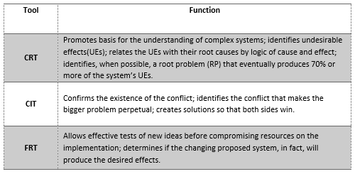
Source: Compiled from Cogan (2007)
Table 2. TOC tool, usual problem solution.
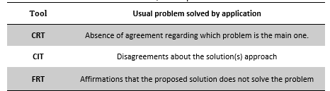
Source: Compiled from Bergland (2016)
2.2 Computational simulation tool
The simulation process can be understood as an attempt to understand an object of study looking at its peculiarities in different levels of abstraction detailing it, and transforming them into a computational model.
“Simulation is a numerical technique for performing experiments on a digital computer, making use of graphics, animation and other technological devices, that involves certain types of mathematical and logical models that describe the behavior of a system (or any of its components) during a particular time” (De La Mota et al., 2017, p.2).
The main idea of modeling is to solve problems that already exist in the real world. The models that are created are always less detailed than the original systems (that exist physically) on which the models are inspired; the modeler has to decide which parts of the system have to be included in the model and which ones not. Modeling is used in situations where tests of possible scenarios are to be carried out because direct changes in the physical system might be too expensive or too difficult (Grigoriev, 2016).
The selected tool for project modeling and simulation was the software called Anylogic® developed by The Anylogic Company. The software is a multi-paradigm tool that supports modeling and simulations based on agents, discrete events and system dynamics.
The three different simulation paradigms differ basically on their abstraction levels, which means that the models can be more or less detailed. The system dynamics paradigm provides models with the highest levels of abstraction and this kind of models is usually applied in strategic situations. Discrete event models are usually applied in situations with low or medium levels of abstraction. Between the previous two modes of modeling there are agent-based models. Such types of model can vary widely in terms of abstraction level, varying from reality-precise models to very generic ones (Grigoryev, 2016). Figure 1 demonstrates the differences between the three paradigms.
Figure 1. Simulation paradigm differences
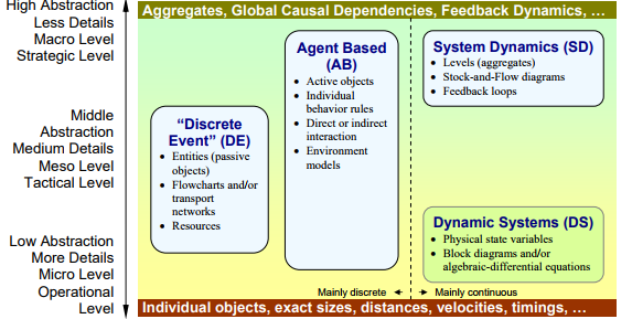
Source: Borshchev et Filippov (2004)
Two areas can be cited as the common fields that use the DES approach of simulation; they are manufacturing and logistics (Rangel et al., 2016). Given the nature of the problem that involves both manufacturing and logistic areas of the company in this work, simulations were made using the discrete event simulation paradigm (DES).
Computational DES was introduced in the second half of the last century as an important analysis tool for decision support. In 1961, IBM engineer Geoffrey Gordon introduced GPSS, considered to be the first software implementation of the discrete event modeling method (Grigoryev, 2016).
DES is characterized as a type of simulation that has changes that occur in a system at specific stages of the simulation time. These changes are responsible for altering the state of the corresponding system as a whole. The DES paradigm of simulation opposes to the continuous- time simulation modeling paradigm, in the continuous paradigm the system can usually be modeled through differential equations (Loper, 2015).
The most important elements of a DES model are: (1) entities that are elements that move in a block network - these entities can perform activities, be delayed and utilize resources; (2) queues that correspond to regions where entities are delayed so that they can after perform a task; (3) activities that are tasks that can be developed by the entities; and (4) resources that are attributes that entities must have in order to develop some tasks (Brailsford et al., 2014).
3 TOC Methodology application
A survey was made with the targeted company employees that worked directly or indirectly to the product assembly or expedition. The considerations of the survey regarded the case of the most complex product assembly (the one that had more assembly stages in the production line). The questions made on the survey aimed to identify the undesirable effects (UEs) of both production and expedition sectors of the company, which were considered the bottleneck to reaching the settled goal.
Eleven (11) UEs were considered in the survey, all being candidates to be the bottleneck of the production and expedition fluxes. The effects were classified according to how much they affected attainment of the goal. Each interviewee attributed a score for each effect; the Likert scale was used as tool for the implementation of the survey. In the case of an effect receiving one as score, it meant that the effect was considered one of great impact in the attainment of the goal, and if the effect received a score of five, it meant that this effect was not relevant when it came to the achievement of the goal.
Table 3 shows the list of effects and their final score after being statistically treated considering the variable scores that were attributed to each effect by each interviewee.
Table 3. UEs obtained score and description of the effect.
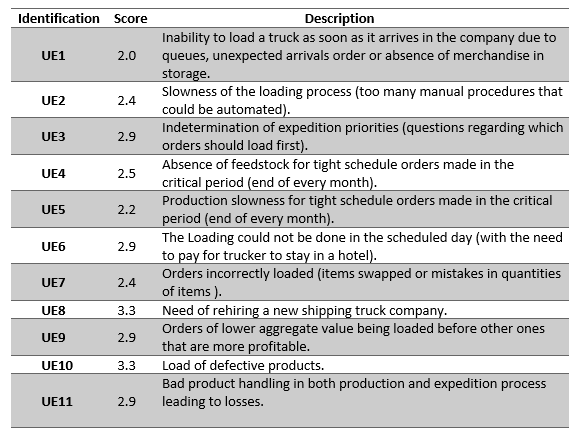
Source: The authors’ own.
Table 3 shows that the effect that got the lowest score (and therefore considered the most relevant effect), responsible for more than 70% of the UEs, was UE1. Based on this effect, the CRT was built and is shown in Figure 2.
Table 4 provides a detailed explanation of the CRT, elucidating the interactions between the undesirable effects, using cause and effect logic, meaning that one effect or the interaction between two or more effects can generate another effect.
Figure 2. CRT regarding the UEs of the manufacturing and expedition system of the company
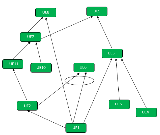
Source: The authors’ own.
Table 4. Cause effects relationships illustrated in the CRT.
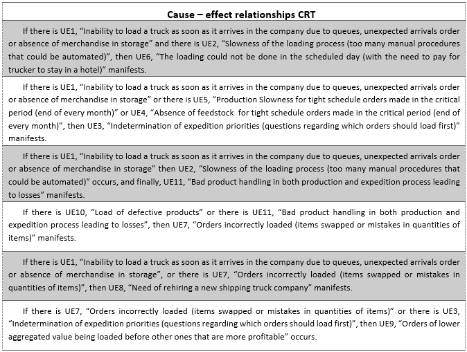
Source: The authors’ own
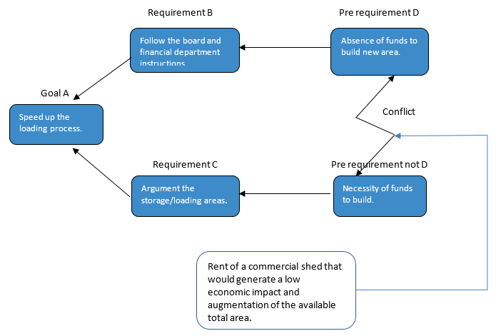
The CIT of the root UE is shown in Figure 3, the injection obtained through the analysis of the undesirable effect will be the entry variable for the creation of the FRT.
Figure 3. CIT used to obtain the DE related to the root UE.
Source: The authors’ own
Figure 3 shows that the goal attainment has two requirements: The first one is that the recommendations of the company’s directive board and financial department are respected, the second one is that the storage and loading areas are increased, creating more space for merchandise to be loaded as well as making the loading process more agile, thus decreasing the truck line at the final periods of each month when there is accumulation of orders.
When the pre-requirements of both requirements are analyzed, it is noticeable that there is a conflict, given the fact that to meet the first proposed requirement (requirement B), the company’s board orientations must be followed, and the recommendation in this case was that there would be no funds to build a new storage and loading area; however, the pre-requirement of requirement C was exactly that a fund had to be raised in order to build such area.
With the intention of finding a solution to the conflict, where the interests of both parts are met, then by eliminating wrong assumptions and ensuring that the root EI is eliminated respecting both established requirements, an injection was proposed and was stated as: rent of a commercial shed that would generate a low economic impact and augmentation of the available total area.
Figure 4 shows a table with the Desired Effects (DE) that are obtained when the UEs are eliminated, to perform such transformation injections are needed (one central injection derived from the CIT resolution that acts on the root UE, and four others that were considered necessary to eliminate some of the non-root UEs). With the application of all injections in the CRT, the FRT is obtained and shown in Figure 4.
The FRT corresponds to an optimal state for both expedition and manufacturing facilities, representing in this case study a virtual scenario where all the problems that occur at the end of every month that come from the accumulations of orders by the company clients are eliminated.
Figure 4. DEs, proposed injections list and FRT of the generated DEs obtained after the application of the five injections.
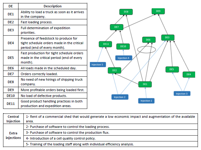
Source: The authors’ own
With the identification of the root UE and the definition of the needed injection associated with this UE, two simulation models have been created, using the Anylogic® simulation software: The first one (S1) brought the current state of the expedition system of the company and the second one (S2) showed the aimed state of the expedition system of the company, after injection one was applied.
4 Model simulation
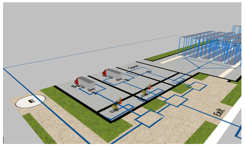
The created environment for the simulation (plant) of the model, after injection 1, is shown both in two-dimensional (2-D) and in three-dimensional (3-D) perspectives in Figures 5 and 6. The environment for the simulation model before the injection (current state) is similar to the one shown in Figure 5 as a 2-D perspective, the only difference being that, it does not have the rectangle in the right part (the one that has only one spot).
Figure 5. Two-dimensional visualization of the developed plant scheme.
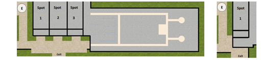
Source: The authors’ own
Figure 6. Three-dimensional visualization of the developed plant scheme.
Source: The authors’ own
The plants are used to simulate the trucks loading process, giving consideration to loading times, slowness in the lines that are formed previous to the entrance (represented by the letter “E” in Figure 5), the selection of the ideal spot (considering the possible options in each simulation model), maneuver times of the trucks, month period of the simulation, day of the week, time of the day, and limit “patience-time” of a trucker before giving-up loading.
Considering the UE1, a supplementary area of loading and unloading would bring improvements to the current problem. The DE8 and DE9 represent measurable quantities that are going to be evaluated directly in simulation. The resolutions that come after the specific case of DE8 are unfolded into two different possibilities: The settling of a new contract (what happens in most cases) or the loss of the sale due to client’s desistence (what generates a considerable loss of both value and volume). The occurrence probability of both cases has been estimated and it is considered in the simulations.
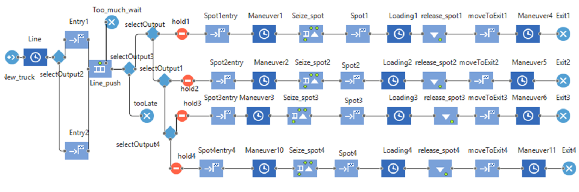
Figure 7 shows the blocks used to make the simulation model of the after-injection state at the company; the used entities are trucks that enter, are loaded and leave the expedition area of the factory. The three flux ramifications correspond to the three spot places available at the company’s truck parking lot.
Figure 7: Block diagram of the DE modeled system.
Source: The authors’ own
In Figure 7, a new entity is created at the block “New_truck”, the entity stays a variable time in the entrance line given by triangular probabilistic distribution (TPR), after that, it goes to the entry point where it stays in the line for a period given by another TPR. If it stays there for a too long period time it abandons the flux throughout the block “Too_much_wait”.
If the entity does not abandon execution, the entity enters the select output area where, if the entry time of the entity is in the expedition working hours range, the entity goes to one ramification where it will be loaded and leave the simulation (trough one of the exit blocks). If the entry hour of the entity is not in the expedition working hours range, the entity will abandon the simulation without being loaded trough the block “Too_late”.
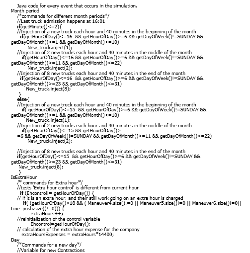
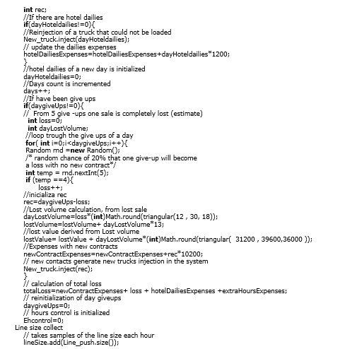
Code in Java language was used (see appendix) to provide logic to the processes that occur in the simulation time. Four cyclic temporal events also take place in the simulation and are responsible for several tasks, such as changing the entities intensity flux, updating execution variables and making calculations regarding the update of such variables. The two simulation models have the same cyclic temporal events with identical codes.
The first event is responsible for changing the flux magnitude depending on the month period, this event occurs daily (except on Sundays), in a cyclic way, it injects trucks from 6:01 to 16:01 in simulation time at each hour and forty minutes in different intensities, depending on the month period.
The second event analyses whether the expedition employees are working on extra hours. That event also occurs in a cyclic fashion at each minute of the simulation and verifies if there is activity in the penultimate blocks of the simulation.
The third event updates the output variables of the simulation and resets daily control variables associated. The last event is used for taking samples of the line size; the samples were taken at each hour of simulation.
To provide a much more detailed explanation of the simulations, and to show the discrete event simulations in real time, two videos have been recorded. The links (paths), of the recorded videos for the worldwide computer network (internet) are given bellow; the password to get access to their content is the same in both the cases: "Bjopm2017“, with URLs:
● https://vimeo.com/246162513 (first simulation video).
● https://vimeo.com/246165575 (second simulation video).
4.1 Simulation results
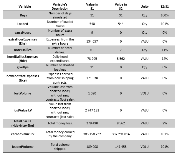
After the creation of the blocks and code insertion, the two simulation models were executed (five hundred and five times each, considering the stochastic nature of the modeled system), and the results of the medium readings of the output variables of all the simulation executions after one month (in simulation time) are shown in Table 5.
With the interest of testing the convergence of the five hundred and five results (obtained for each variable) on each simulation and following Freitas Filho (2008) orientations, confidence intervals were measured for the variables of the earned value, loaded volume and total loss of the system and a precision level was set as five per cent, for each of those variables, meaning that, if the confidence intervals represented five per cent or less of the arithmetic mean value of these variables, no further simulations are required.
The output variables are presented one by one and their final mean values in the first and second simulations for a period of one month in simulation time. All the variables are initialized in the beginning of each simulation with zero value; the length of a month simulation is equal to 31 days. To guarantee the confidentiality of the gathered data, the units used for volume and money revenue measurements are named as reference expressions VALU (value unit) and VOLU (volume units); those units do not correspond to any standard unit system.
Once all simulations were concluded, a quotation for a shed rent value was made. Rental costs, along with the maintenance expenditures, energy supply, transportation of loads between the storage units, and expenses with the hiring of new employees have represented fewer losses when compared to the first simulation losses.
Table 5. Comparisons between variables outputs (using arithmetic means of all executions) in the two created simulation models.
Source: The authors’ own
The precision levels obtained in the first simulation model were 0.07%, 0.07%, and 2.45 % for the variables earned value, loaded volume and total loss, respectively, and 0.08%, 0.07% and 4.38% for the same variables in the second simulation model; therefore, the requirement of convergence was met and no more simulations were considered necessary.
The company's profit derived from the shed's rent can be calculated as the difference between the differences obtained by the subtraction of the company's earned value (EVS2 and EVS1) and the total losses of each model of simulation (TLS2 and TLS1) minus the new shed's rental and maintenance monthly expenses (NS), which were quoted as 1,000,000 VALU, the result of the calculation was 3,503,710 VALU which represents more revenue to the company. This revenue is represented by the variable CP (company's profit). Equation 1 describes the previous stated calculation.

where,
CP: company’s profit [VALU]
EVS2: Total earned value in simulation model 2 [VALU]
TLS2: Total loss in simulation model 2 [VALU]
EVS1: Total earned value in simulation model 1 [VALU]
TLS1: Total loss in simulation model 1 [VALU]
NS: New shed monthly expenses [VALU]
For each simulation model, a chart was plotted regarding every truck that was loaded and total loading time in the line, those charts are presented in Figure 8 and are arithmetic means of the five hundred and five executions of each simulation model.
Figure 8. Trucks loading time for each truck in simulation 1 (left) and simulation 2 (right).
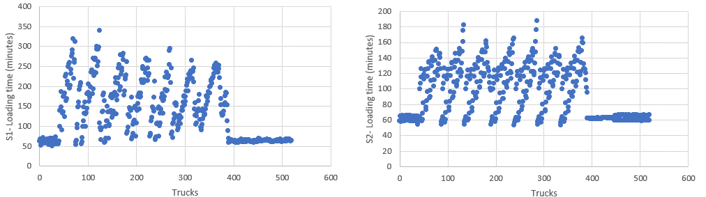
Source: The authors’ own.
In the first simulation, the maximum loading time (including the time spent in the trucks line) of a single truck was 340 minutes and the average loading time of the loaded trucks was 134 minutes. In simulation model 2, those values were 188 and 96 minutes, respectively.
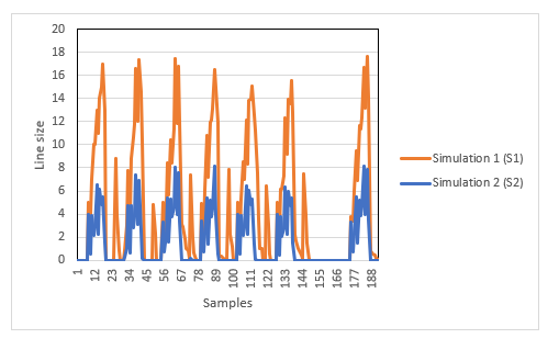
Figure 9 represents the line size in the entrance of the expedition area. For each hour of simulation (in the critical simulation period that corresponds to the end of the analyzed month) one sample of the line’s size was taken with the intention to diagnose how many truckers were forming a line in both simulation models.
The values between samples were interpolated to generate a continuous chart. In the first simulation, the peak value of the trucks in the line was eighteen trucks, and the mean line size length was five trucks. Those values were eight and two in the second simulation, respectively. All results described (and presented on figure 9) are arithmetic mean results of the five hundred and five executions of each simulation model.
Figure 9. Line size at each hour of simulation for S1 (orange) and S2 (blue).
Source: The authors’ own
In figure 9 the long sample span (between samples 147 and 172) that has registered 0 as the value of trucks in both simulation models, corresponds to a Sunday in the simulations. Sunday is a day in which there are no workers in the loading area of the company and, therefore, there is no trucks injection in the simulation.
From Figures 8 and 9 and using the mean and peak values for each simulation model, it is clear that the rent of a new shed would represent a better scenario for the line of trucks.
5 Final considerations
The work contained in this document was developed, considering a pet care company that had a specific goal for its production and expedition sectors that was augmenting its availability of products in the final periods of each month for immediate shipping. The authors of this study have chosen a theory of the constraints combined with discrete event simulation analysis in order to generate solutions for the attainment of the company’s goal.
Aiming to verify the usage of this combined approach in other works, two searches were made in web databases. The conclusion of the research was that the combined approach of methodologies has not been applied frequently on management related discussions and, therefore, the solutions contained on this work hoped to deepen this type of discussion.
The development of the analysis was oriented firstly by the process of gathering data from within the company, a survey was made with employees and, after the results of the survey were obtained, the bottleneck that was a hindrance for the goal’s attainment was identified with the application of the theory of constraints tools.
The bottleneck identified in this case study was in the expedition sector of the targeted company. The conclusion of the application of the TOC methodology was that, although the company frequently has the products required by its clients (distributors) in the higher demand periods, these products often cannot be loaded in able time generating a revenue loss.
With the bottleneck identification and having information about the company’s infrastructure and processes’ sequence of its expedition sector it was possible to create a model that could represent the expedition sector and the procedures that were carried out in this part of the company.
After the models’ creations were made, simulations were done through Anylogic®, comparing the current scenario of the company and the virtual scenario posterior to the application of the central injection, which was proposed after the TOC analysis was made. It is shown that the latter scenario was proven to be more profitable and organic regarding the availability of products to be loaded when the demand intensifies as the last section of this work brought numerical comparisons between both scenarios showing the advantages of the second scenario.
Additional analyses were made in order to show the differences of truckers waiting times in the waiting lines of the company and the loading time duration span, those results were plotted in chart forms and have also showed clear advantages when the proposed modifications (corresponding to the second simulation model) were adopted.
The work has presented a practical analysis of a classical theory of production engineering; results have been gathered and discussed. The applied methodology is recursive and algorithmic, considering the ongoing improvements that most private capital company’s use today. Furthermore, the analysis can be reapplied looking for a constant refinement to the purpose of reaching the selected goal.
References
ABINPET (2017), “Faturamento 2016 do setor pet aumenta 4,9% e fecha em r$ 18,9 bilhões, revela ABINPET”, available from: http://abinpet.org.br/site/faturamento-2016-do-setor-pet-aumenta-49-e-fecha-em-r-189-bilhoes-revela-abinpet/ (Access: 6 May 2017).
Bergland, E. (2016), Get it done on time! A critical chain project management/theory of constraints novel, 1st ed., Apress, Redwood City.
Borshchev, A.; Filippov, A. (2004), “From system dynamics and discrete event to practical agent based modeling: reasons, techniques, tools”, paper presented at The 22nd International Conference of the System Dynamics Society, Oxford, OXF-UK, 25-29 July 2004, available from: www.anylogic.ru/upload/iblock/296/296cb8fa43251a1fc803e435b93c8ff2.pdf (Access: 08 Sep 2017).
Brailsford, S. et al. (2014), Discrete-event simulation and system dynamics for management decision, 1st ed., Wiley, Chichester.
Cogan, S. (2007), Contabilidade gerencial: uma abordagem da teoria das restrições, 1st ed., Saraiva, São Paulo.
Cox III, J.; Schleier, J. (2013), Handbook da teoria das restrições, 1st ed., Bookman, Porto Alegre.
De La Mota, I. et al. (2017), Robust modelling and simulation integration of simio with coloured petri nets, Springer, Cham.
Freitas Filho, P. (2008), Introdução a Modelagem e Simulação de Sistemas com Aplicações em Arena, 2nd ed., Visual Books, Florianópolis.
Goldratt, E.; Cox III, J. (2004), The goal a process of ongoing improvement, 3rd ed., The North River Press, Great Barrington.
Grigoryev, I. (2016), Anylogic in three days, 3rd ed., available from: http://www.anylogic.com/upload/al-in-3-days/anylogic-7-in-3-days.pdf (Access 26 November 2016).
Loper, M. (2015), Modeling and Simulation in the Systems Engineering Life Cycle, 1 ed., Springer, London. Rangel, C. et al. (2016), “Discrete-event simulation models for didactic support”, Brazilian Journal of Operations & Production Management, Vol.13 No.3, available from: https://bjopm.emnuvens.com.br/bjopm/article/view/V13N3A7/BJOPMV13N3A7 (Access: 10 September 2017).
Santos, R. et al. (2010), “A real application of the theory of constraints to supply chain management in Brazil”, Brazilian Journal of Operations & Production Management, Vol.7 No.2, available from: https://bjopm.emnuvens.com.br/bjopm/article/viewFile/V7N2A5_/V7N2A5 (Access: 03 September 2017).
Watson, K. et al. (2007), “The evolution of a management philosophy: The theory of Constraints”, Journal of Operations Management, Vol. 25, pp. 387–402.
Appendix
Java code for every event that occurs in the simulation.
Received: Sept 15, 2017
Approved: Jan 12, 2018
DOI: 10.14488/BJOPM.2018.v15.n1.a6
How to cite: Barbosa, G. L. L.; Cooper, R. E.; Anholon, R. et al. (2018), “A manufacturing bottleneck case study trough the theory of constraints and computational simulation of the proposed bottleneck solution”, Brazilian Journal of Operations & Production Management, Vol. 15, No. 1, pp. 54-67, available from: https://bjopm.emnuvens.com.br/bjopm/article/view/399 (access year month day).