Application of Agent Based Simulation to analyze the impact of tax policy on soybean supply chain*
Carlos Henrique Viégas De Rosis
carlos.rosis@gmail.com
University of São Paulo, São Paulo, São Paulo, Brazil.
Marco Aurélio de Mesquita
marco.mesquita@poli.usp.br
University of São Paulo, São Paulo, São Paulo, Brazil.
*The results of this research have received significant
contribution from Dr. José Roberto Castilho Piqueira (Poli USP)
ABSTRACT
This work seeks to explore and demonstrate the use of Agent Based Simulations (ABS) in modelling and simulating supply chains. Such methodology was applied to develop a model to evaluate the impact of current tax policies in soy supply chain in Brazil. The model brought interesting insights on how the country’s current tax structure induces logistics and tributary trade-offs, therefore generating a suboptimal grain distribution. This is accomplished by going through the conception and implementation of an Agent Based Model. First there is the definition and delimitation of the main agents acting upon soy’s supply chain, such as producers, trader and consumers. Those agents then have their behaviors studied and translated into programable patterns. Finally, the model considers the environmental interactions with the mentioned players, including the effects of infrastructure capacities, transportation costs, storage costs and tax legislation. After quantitative and behavioral validation, the simulation is then able to mimic the actual allocation of corn, soy and soymeal productions in their respective supply chains. This would allow inferring how the system could work in different tax conditions, thus quantifying the tributary impact in terms of congestions, idle infrastructure and delays. The analysis of such results points out that a path dependant tax system may induce agents to opt for inefficient logistic solutions, if such alternatives are cheaper when taking taxes into account. From those simulations it is possible to conclude that there are opportunities for supply chain efficiency gains in the design of a new tax policy.
Keywords: Agent Based Modelling and Simulation; Soy; Corn; Supply Chain; Supply Chain Modelling.
1 INTRODUCTION
Agent Based Simulation (ABS) is a relatively new class of computation models – if it is compared to other simulation approaches, such as Dynamic Systems and Discrete Events – and there is still no consolidated approach concerning this tool. Nevertheless, it has proven itself useful and it is growing in the engineering field (Klügl, 2016). It works through the observation of the emerging behaviour of a complex system composed by many autonomous and interacting individual entities (Macal & North, 2010). This mechanism makes ABS a useful tool for the decision making process in environments where the decision maker has low control over all agents in the system. A good example for the application of such method would be public policies design, because it allows the simulation of the behaviors that multiple stakeholders may have under a new policy or regulation, determining the policy success and additional effects.
In the aforementioned context, the goal of the present work is to explore the Agent Based Modelling and Simulation framework, reproducing and demonstrating the methods proposed by Klügl (2016) and Macal & North (2010) in order to provide insights concerning public policies in the agriculture sector. This was done by applying Agent Based Simulation to model and simulate soy and corn supply chains aiming to evaluate the impact of the current tributary policy in Brazil’s soy trade. Therefore, this study was able to simulate public policies concerning some of the most important sectors in the Brazilian economy, such as soy and soy meal, which accounted for 53% of all Brazilian agriculture exports in terms of weight in 2015 (ANTAQ, 2015).
Besides its great importance, this sector faces major challenges concerning logistics and supply chain efficiency due to a trade off in between optimal logistics and taxation. Those challenges are exposed in the studies conducted by Santos and Abrita (2016), which indicate that soy export’s tax exemption and the current Brazilian tax configuration generate negative externalities in the soy supply chain, deindustrializing the sector and increasing processing plants’ idleness. This situation happens because soy and soy meal trades, involving agents located in different states, are penalized in detriment of exports.
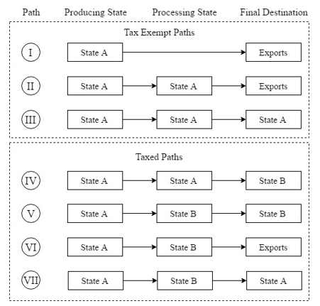
The mentioned tax’s path dependency is better exemplified in the diagram bellow, where there are different possibilities for soy to be processed or exported after being produced on state A. This diagram shows the path dependency in the tributary system because, even though there are paths with the same end result (i.e.: III and VII finish with soy being consumed at State A and II and VI end in exports), they are taxed differently. Such situation generates inefficiencies, because, even though the taxed paths might sometimes be more logistically efficient, they are not going to be used due to their extra costs. This scenario creates a trade-off in between optimum logistics and taxation, therefore producing unbalances in the supply chain, incentivising excess and scarcity of soy and soy meal to coexist across state’s borders.
Figure 1. Description of the tax mechanisms in the soy supply chain
The situation shown above indicates that, at least theoretically, there is a great opportunity in terms of public policies because the entire sector would be more efficient with an improved taxation. However, in order to design such measure, it is necessary to estimate how agents act under different tributary rules and, then, evaluate how the system’s efficiency would change under such conditions. For this purpose, the model in this work replicates each agent’s behavior in the soy supply chain, such as producers, traders, consumers and ports in a georeferenced network subject to infrastructure constraints, freight costs, government taxation, and regulation. Moreover, it also considers the effect of corn supply chain due to mutual interference in infrastructure use and congestions. Finally, the model is used to evaluate how the system is affected in terms of soy processing plants’ utilization, logistics costs and infrastructure congestion if taxes cease to be path dependant. Therefore, this model can be useful in the governmental decision making process because it estimates how autonomous agents in the agriculture sector react to a tributary policy in terms of supply chain efficiency.
To demonstrate this idea, this article is structured in six sections. First, this work reviews theoretical concepts concerning agent based modelling in the theoretical background section. The next section describes the methods used to model and analyse soy supply chain under different tributary scenarios. The modelling section shows the application of such methods, presenting the model development and implementation. Next, the fifth section presents analysis and the model validation. Finally, the last section summarizes the article and draws its final conclusions.
2 THEORETICAL BACKGROUND
This section synthetizes the theoretical background concerning Agent Based Simulation and its application to the taxation in the soy supply chain. First, it goes through a review of agent based modelling and simulation tutorials in order to build the framework presented in this work. Second, it visits other works concerning supply chain simulations, indicating trends and presenting Agent Based Simulations applied to such kind of problems.
2.1 Agent Based Simulation
Even though there are no consolidated modelling practices in ABS, Klügl (2016) and Macal & North (2010), have presented structured approaches, guides and tutorials towards building agent based models and simulations. These approaches were useful in order to conceive and develop the simulation model shown in the next section. Those two approaches are quite similar and can be summarized in three steps:
• Definition of the agents
• Definition of interactions and topology
• Environment definition
The conception of a model starts after the definition of a problem with variables of interest. In the context of an agent based model the first step would be to study the underlying problem in detail in order to define and delimit the objects which have influence over the problem’s outcome. These entities are usually active and autonomous in respect to the other agents in the simulated environment. Each agent may have a set of static or dynamic attributes representing the entity’s characteristics, such as age, income, gender, beliefs, inventory level, etc.
In this second step, definition of agent’s interactions and organization, each one of the previously defined agents is observed. The observations are then used to understand and represent the drivers and rules permeating the agent’s behavior and their relationships. Those drivers and rules can be represented in many ways: a Nash Equilibrium, and animal instinct, any pattern found in behavioral economics, or a cultural convention. In addition, it is necessary to understand the relationships and communication in between agents, which can be represented, for instance, as a network, a cloud or a set of free objects moving through space.
Finally, it is necessary to define the environment underlying the entire model. This step consists in understanding and representing the interactions in between the agents and the environment as they might be mutually influential. Even though the environment is usually an inactive object, as the agents, it also may have parameters such as pressure, color, luminosity, etc.
2.2 Agent Based Simulation applied to Supply Chains
In addition to the visited Agent Based Modelling and Simulation (ABMS) framework, it is also useful to verify the use of Agent Based Simulations applied to supply chain management. Van der Zee & Van der Vorst (2005) have perceived the opportunity in the uses of methods which would present explicit control structures, focused on controlling agents, instead of methods focused on physical transactions and processes. Since then, ABMS has grown rapidly and continues to evolve due to the development of new approaches and techniques such as the model calibration framework presented by Magariño & Navarro (2016). Moreover, ABMS frameworks have made significant progress towards simulating human behavior and decision making process. Elkosantini (2015), for instance, proposes a generic simulation model for human centred simulations.
Concerning supply chain simulations, the literature review made by Oliveira et al. (2016) indicates that agent based models are becoming an increasing trend in the supply chain simulation field and is expected to grow because such method has emerged as a robust and competitive tool for modelling highly complex interfaces in supply chains, where other methods such as DES are currently more used. While DES is especially useful to simulate certain elements of a supply chain, such as a port terminal Cimpeanu (2014), ABMS is a very powerful tool when the simulation reaches a wider scope. An interesting example is the work conducted by Dorigatti et al. (2016), where a generic, versatile and systematic method is presented to model and transport interactions in supply chains is simulated using an agent based approach.
In this work, Dorigatti et al. (2016) presents three kinds of agents: Client, Transport and Supplier. Both Client and Supplier are arranged in a georeferenced network while Transport moves from one agent to the other. In terms of behavior, all agents exchange information such as demand requirements and sourcing plans in an iterative form, generating a delivery plan, a distribution plan, a production plan and a sourcing plan. After agreeing upon such plans, the supplier starts to fulfil the orders in the plans by verifying the inventory and sending the products to the Client through the Transport agent; the Client receives the order and informs the Supplier. If events, such as expired products, stock out at the supplier or the Transport agent is unavailable, the order is cancelled. Finally, the model takes into account environmental elements such as distances in between Suppliers and Clients.
3 FRAMEWORK DEFINITION
Before applying the agent based model framework to the analysis of logistics and supply chain efficiencies in the grain sector, it is necessary to first demonstrate whether such method is suitable to the grains supply chain modelling and simulations. The main reason to endorse such method for this application is the direct correspondence in between real life and the agent based model elements. For this reason, it is relevant to indicate the presence of agents such as grain producers, traders, logistic operators, cooperatives and grain consumers responsible for decentralized decisions that affect the system’s overall behavior. Those agents have a well-defined decision pattern, as they take actions in order to maximize their profits. In addition, there is an environment which subjects the agents to a transportation network possessing dynamic and static properties such as congestion levels, tax legislation and infrastructure capacities that influence agents’ decisions.
After indicating the possibility of the application of such method to tax policy in the grain supply chains, the application of this framework follows guidelines close to the ones presented in the last subsection. First, this work reviews some concepts regarding soy and corn supply chains in Brazil in order to gather information on its main agents and their relationships. Next, there is the definition and delimitation of the main players in this environment, which is used to shape a conceptual model, describing the model’s topology and agent’s interactions in a generic supply chain, similar to the one presented by Dorigatti et al. (2016).
Then, each agent and each supply chain is further studied and differentiated from the others according to the used commodity. In addition, the agents’ behaviors are translated in programmable patterns, modelling price formation, material flows and communications. Finally, the model considers other environmental factors such as distances and transhipment costs.
Those patterns defining each agent’s behaviors are then implemented in python. It generated a model that was inputted with data containing parameters such as consumers’ demand, freight prices, taxes, grains’ seasons and local amounts produced, etc., collected and estimated from institutional and governmental databases. Next, the model was validated by confronting the model’s outputs with historical data such as exports, grain balances and processing industry utilization rates. Moreover, the hinterlands presented in the model shall be compared to the actual hinterlands and existing infrastructure.
After the validation, the model underwent a scenario analysis which compares the current tax system to other in which taxes are not path dependent, thus, not generating trade off in between optimal logistics and optimal taxation. In this new scenario, indicators involving soy processing plants utilization and congestions at ports were used to evaluate the outcomes of a non-path dependant tax system.
4 FRAMEWORK APPLICATION
This section starts by reviewing some concepts concerning grains supply chain that are utilized to build an initial prototype. This first prototype, based on qualitative information, seeks to reflect agents’ behaviors and grains supply chains configurations, translating them into programmable patterns. Then, it is further detailed over the following sub sections, receiving both quantitative and behavioral inputs, resulting in a final simulation model. Its results are then discussed, validated and analysed on section five, providing evidence for the conclusions drawn in the last section.
4.1 Grains Supply Chains overview
The literature presents many works that map the agents in the soy and corn supply chains in a regional and national context, defining their interactions and organization. Roberti et al. (2016) show the soy supply chain defined by five players: inputs suppliers, producers, originators, processing industry, and final consumers. The first are the providers of seeds, chemicals, fertilizers and equipment. The producers use those inputs to plant and harvest soy, the originators buy the producer’s grains and conduce the distribution process (storage and transportation). The processing industry transforms soy into soy meal and soy oil, and finally, the final consumers are mostly the livestock industry, and soil oil to produce biodiesel or use in the food industry and households.
Other authors such as Machado et al. (2013), and Silva et al. (2010), also present a similar configuration to the one mentioned above. In addition, Martha Junior (2012) provides a similar model to represent the corn supply chain, consisting of: suppliers, corn producers, originators, processing industry and final consumer. Figure 2 shows a summary of the agents and their relationships in the aforementioned works in both supply chains.
Figure 2. Soy and corn supply chains agents and their interactions
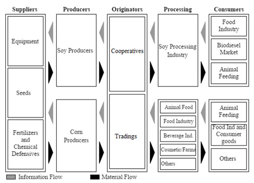
The previous diagram is useful to observe behaviors and create a first version of a supply chain model, in the next subsection. It shows the material flows, given by agriculture inputs, grains or their sub products, and information flows, given by cash, future contracts, or prices, exchanged among agents.
4.2 Model overview
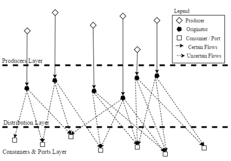
According to the material and information flows observed in the Figure 2, in the last section, there are direct correspondences in between the agent’s position in the supply chain and behaviors, such as: players can act as distributors, producers, consumers, or a combination of those roles for a given product. These players can be represented in a network with multiple layers, where each layer groups a certain class of agent according to its geographic position, as the one presented in Figure 3, bellow:
Figure 3. Conceptual Model Prototype
Agents
According to the conceptual model prototype, there are three types of agents: First, there are the producers, characterized by an endogenous curve of production over time, simulating the harvests or output of the processing industry, this production flow is, then, allocated to nearby traders, which will distribute the commodity across ports and consumers by evaluating the trade off in between logistics costs and prices paid by each entity. Finally, ports and consumers will present a price curve, which is related to each agent current inventory level, consumption rate and seasonal factors. In addition, it is important to notice that the processing industry is not represented by a single individual agent because it can be represented by a consumer of soy and a producer of soy meal, where the exiting flow of soy meal is conditioned by the inventory level and the incoming flow of soy.
Agents Behavior and Topology
Proceeding with the defined method, this subsection should define the behaviors and configuration of each one of the previously defined agents using a programmable pattern, taking into account each agent objective. First, there are the producers which either have an endogenous production curve (i.e.: soy and corn farmers) or have a steady production which depends on the presence of inputs (i.e.: soy processing plants for soy meal). Second, there are the traders, which will continuously evaluate commodity prices and freight costs and then will send products to the most profitable consumers. Finally, there are the consumers, such as processing plants, cattle and chicken breeders and ports, which will value inputs based upon current stocks and external factors.
Producers
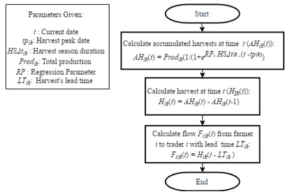
There are two kinds of producers in terms of behaviors; farmers and soy processing plants. The first algorithm, presented on figure 4 bellow shows how farmers behave. They have a predefined endogenous production curve based upon the products’ seasonality and historic production; this production is then transferred to a trader after a lead time 〖LT〗ik, where i is the producer’s index and k is the crop index. The accumulated production is represented by a sigmoid curve centred in the harvest season peak and is parametrized according to the harvest duration as to represent its seasonality.
Figure 4. Soy and Corn producer's behavior algorithm
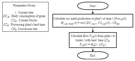
The second type of producer, the soy processing plants, have a fixed operation capacity, given by its equipment. In this context, if soy is abundant, it should have a stable soy meal production close to its total capacity, otherwise, if inventories are depleted, soy meal production should be zero. Moreover, as the farmes, the soy processing plants have a lead time to send its soy meal to an originator. The processing plants behavior is represented in the algorithm bellow.
Figure 5. Soy processing plant's behavior algorithm
Originators
In the model proposed in this work, the trader’s behaviors were inspired by the Congestion Game. This game, as introduced by Rosenthal (1973), is a game in which each player should choose to use one or more resources from a set of common resources. The payoff function associated with each resource and player is a decreasing function, depending on the number of players using that very same resource. In such way, a congestion game is a suitable model to represent decisions made under scarcity of common resources.
Concerning this simulation, originators would be constrained by the scarcity of resources such as ports capacities or local consumer’s demand. Therefore, each of the agents would weight freight and price of the commodity before choosing where to sell their products at every simulation step. This behavior is comparable to an iterative best response algorithm if the model assumes atomic players acting in a sufficiently short time interval. It happens because it takes multiples iterations before a significant change in routes and prices conditions occur. Therefore, we have the following solution for the trader’s flows of a generic commodity in the position i and linked to the consumer j at time t represented in the algorithm in Figure 6:
Figure 6. Originator's behaviors algorithm
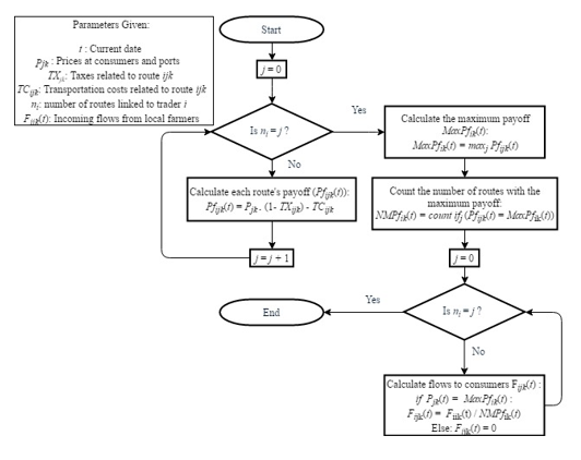
According to the algorithm above, each trader will evaluate the prices practiced at each consumer and then calculate each route’s payoffs by considering freight costs (and taxes). The trader will then divide the incoming flow from farmers equally among the most profitable consumers and will send nothing to the remaining consumers.
Consumers and Ports
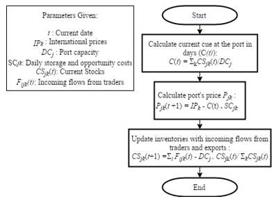
Proceeding to the last set of agents, there are the consumers and ports algorithms represented in figures 7 and 8 bellow. These agents have very similar behavior, as they divulgate prices to adjacent traders in order to influence incoming commodity flows and then update their inventories. The mentioned agents also have an exit flow representing the consumers demand rate or the ports capacities. The only difference among the mentioned players are the functions defining their prices. The consumer’s prices are defined as a sigmoid function, considering the difference in between their current inventory position and the expected inventory, given by a seasonal curve. Otherwise, prices at ports are given by the total storage costs subtracted from the commodity prices practiced internationally. In this case, the total storage costs would be given by the current inventory position (in days) multiplied by the unitary storage costs.
Figure 7. Consumers' behaviors algorithm
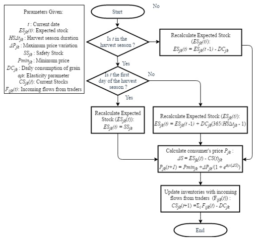
The consumers will compare their current inventories to their expectations, which are given by a crescent linear function during the harvest season and decreasing linear function during the off season. If their inventories are lower than the expectations, prices should be high and low otherwise, obeying a sigmoid function with a minimum value of 〖Pmin〗jk and a maximum value of 〖Pmin〗jk+ 〖∆P〗jk. The maximum value represents the maximum price the commodity is willing to pay for an additional ton of commodity before stopping its operations, while the minimum value represents the price at which the consumer would recognize an arbitrage opportunity, therefore willing to buy an unlimited amount of inputs. In addition, prices sensitivity to inventory variation is given by the αjk parameter.
Figure 8. Ports' behaviors algorithm
Considering all players described above, we have that information (prices) and the modelled commodities travel in opposite directions, stablishing multiple balancing feedback loops, therefore making it difficult for consumers or ports to have excessive stocks or run out of the modelled commodity.
4.5 Environment
Other than the agent’s and their behaviors, there are elements in the model that affect agent’s decisions, such as distances, transportation infrastructure, infrastructure quality, and tax legislation. Those elements are materialized in the form of logistics costs and IVA taxation, prioritizing some routes over others.
In order to calculate players’ payoffs, other than product prices, it is necessary to consider freight costs because in agriculture, as players deal with large volumes of commodities of low aggregate value in business-to-business context, logistic costs and taxes become one of the most important factors in the players’ decision-making process. Therefore, the inputs concerning logistics costs must consider:
• Freight costs through roads
• Freight costs through railroads
• Freight costs through waterways
• Transhipment costs
• IVA
Each one of these inputs is specific across different routes and geographies; therefore, they must be carefully studied before being inputted in the model.
4.6 Consolidated model
Taking in account all studied agents, kinds of crops and behaviors, the model should have the topology presented in the Figure 9 bellow:
Figure 9. Agent Based Model Topology
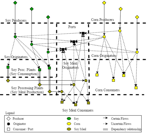
In this topology there are the soy and corn supply chains. The first consists of soy producers that can send their productions to soy processing plants that produce soy meal for animal feeding. The second consists of corn producers that can send their productions to many kinds of consumers (most of it animal feeding). Furthermore, all crops can be exported, causing mutual interference in commodities at ports.
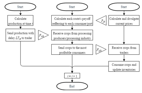
Moreover, Figure 10 bellow shows a summarized algorithm for the model, integrating the behavior algorithms shown on subsection 4.4. It starts by calculating current producer’s production and then sends it to the trader; next, the consumers update the prices, the traders evaluate all routes’ payoffs and send the incoming production to the most profitable consumers. Finally, the consumers will receive the crops, use some of it and update their inventories. The model will then proceed to following time frame. Each time frame consisting of one day and model is run for one year, according to productions and infrastructure conditions of 2015.
Figure 10. Summarized algorithm proposed for the Agent Based Model
5 RESULTS AND ANALYSIS
This section describes the outputs of the model and compares it to historical data to validate it. Those outputs assume multiple dimensions, such as exports by port, exports over time, and geographic influence of each port, proving the model coherence. Furthermore, the differences in between the model and the reality can be explained by other variables with unavailable data or little effect over the model’s behavior (such as infrastructure conditions or weather). This section will also delineate the taxation scenarios that will be discussed in the next section, providing support for this article’s conclusion.
5.1 Model Validation
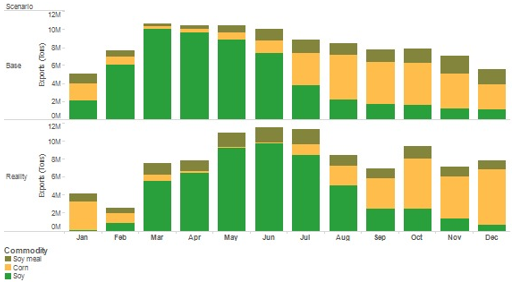
The first variable used to validate the model are the aggregated exports by crop and month, using historical data from official sources (SECEX, 2016) as the main source for validation. In the chart 1 bellow there are the exports according to the model and the exports in 2015 according to official data. Even though both sets of data present the same behavior, it is noticeable that the official data is shifted about two months to the right. This difference can be explained by the fact that the model does not replicate all the lead times in the supply chains. In addition, it does not consider transit time or bureaucracy delays.
Chart 1. Aggregated exports over time by crop
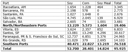
Another way to check the model’s consistency would be to compare accumulated exports by crop and port over the year. In the tables 1 and 2 we can compare this data according to the model and official sources (SECEX, 2015). In this case, both tables show a remarkable resemblance because exports are similarly distributed across ports and crops and the small discrepancies could be explained by commodity prices’ fluctuations, while the model considers international traded prices and freight costs as constant. Additionally, there may be some differences generated by poor infrastructure quality and the presence of logistic synergies, such as the existence of return cargo.
Table 1. Estimated port’s throughput by crop and port
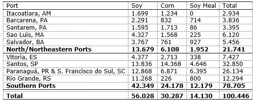
It is important to observe that the tables have unified Paranaguá and São Francisco do Sul ports. This happens because these ports are very close from one another and dependant from the same transportation infrastructure, thus working as if they were one single port and possessing the same hinterland.
Table 2. Real port’s throughputs by crop and port (SECEX, 2015)
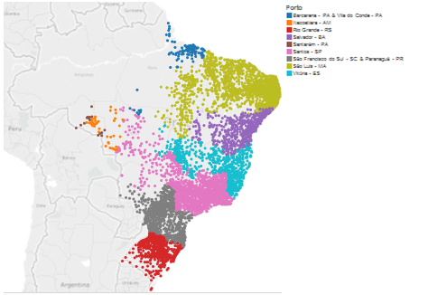
Proceeding to the next validation step, the model with the reality can be compared by observing the most important ports by region. The criteria used to define the hinterlands were the volume of exports in a 300 kilometers radius. Both maps in figures 11 and 12 show similar hinterlands, again endorsing the model’s consistency.
Figure 11. Estimated Hinterlands
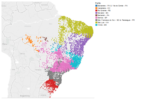
For this analysis, again the ports of São Francisco do Sul and Paranaguá were considered together due to their proximity.
Figure 12. Real Hinterlands
5.2 Analysis
In order to evaluate the effects of IVA tax’s path dependency in the soy supply chain, an additional scenario is going to be considered: a NOTAX Soy scenario, which considers a system where there is no path dependency in the tax system for the soy grains, consequently, taking out the trade-off between taxes and logistic costs. This additional scenario will be compared to the Base scenario in terms of: quantity of soy processed (Chart 2), and congestions at ports, represented by the aggregated quantity of grain waiting to be exported (Chart 3). In those cases, an increase in the soy processing activity is expected, representing a growth in soy processing plants utilization and flatter curve in terms of inventory positions at ports, representing a decrease in the seasonal character of the system.
Chart 2. Comparison of the Base scenario with a non-path dependent tax scenario in terms of soy processing
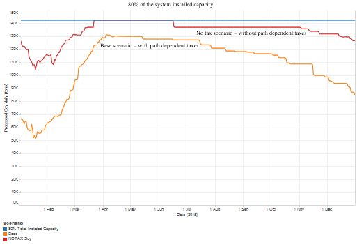
In the Chart 2 above, there is an increase of 23% in the soy processing activity, rising soy plants utilization from 61% up to 75% in the NOTAX Soy scenario. Furthermore, soy meal production becomes more stable as more soy plants work at their maximum capacities for longer periods. In addition, the increase in processed soy should have positive reflexes in terms of ports congestions and transportation demand because the intensification of soy meal production should improve infrastructure utilization during the off season, while peaks resulting from the soy harvest season should be smoothed by the additional amounts of soy being absorbed by the processing plants.
Analysing the ports inventories by product in the chart below, it is observable that the aggregated amount of grains waiting to be exported is dependent on those grains seasonality, having their peaks shortly after the harvests peaks. Nevertheless, there are slight changes in between scenarios in terms of inventory volumes because soy meal has a more consistent presence over time. This situation was already expected due to the increase in soy meal production, seen in the last chart. Moreover, the additional processed volumes of soy should decrease the soy peaks in terms of inventories and the increase of soy meal volume should increase ports’ inventory positions during the off-season, therefore decreasing the seasonal character of exports.
The mentioned situation is better observed and confirmed by the Chart 3. This chart directly compares aggregated ports inventories across scenarios, showing that the export’s valley, in February, is more active during the peak period, from April to October, and it is smoother in the NOTAX Soy scenario. This condition should lower the waiting time for ships to load their grain; however, this is not quantified by the model.
Chart 3. Comparison of the aggregated inventory positions at ports in the evaluated scenarios (tons)
Summarizing the results presented in this chapter, it is possible to indicate that, if taxes ceased to be path dependent for soy grains, the entire supply chain would benefit from this in terms of efficiency in large or small scale. First, the soy processing plants would have a great increase in terms of utilization; second, ports would have less congestion due to the reduced inventories during the peak season and would be less idle during the off seasons.
6 CONCLUSION
Referring to the objective listed in the introduction of this work, this article explores the Agent Based framework, demonstrating how such method can be applied to the evaluation of tax policies’ effects in agriculture. Furthermore, this work presents a structured and formal procedure for developing a complex model, following the guidelines proposed by some authors in the literature. Therefore, the steps used in this work can be replicated in order to aid the development of similar model applied to other problems.
Moreover, the developed model is accurate and robust, providing a picture of the grain supply chains in Brazil under different conditions in a scenario analysis. The multiple outputs of the model, in terms of exports, internal consumption, grains’ flows and routes, show internal consistency. This situation strengthens the recommendation, which indicates an opportunity in using a non-path dependent tax system, which would increase soy processing plants’ utilization and decrease transportation infrastructure’s congestions.
Nevertheless, an Agent Based Model requires a large amount of resources in terms of data and specific knowledge on the system due to its bottom up nature. In addition, this kind of model presents challenges in terms of software and methods because there is no consolidated standard tool or procedure. Still, such models can be really helpful when dealing with complex systems, presenting many active elements with decentralized decisions and behaviors, such as supply chains. Therefore, it is important to develop and consolidate methods and best practices to explore such opportunity.
REFERENCES
Associação Brasileira das Indústrias de Óleos Vegetais – ABIOVE (2016), Tributação na Indústria de Óleos Vegetais, disponível em: http://www.abiove.org.br/site/_FILES/Portugues/18082012-172550-abiove_palestra_camara_setorial_soja_ago11.pdf (acesso em 15 set. 2017).
Agência Nacional de Transportes Aquaviários - ANTAQ (2015), Sistema de Informações Gerenciais, disponível em: http://portal.antaq.gov.br/index.php/sistema-de-informacoes-gerenciais-sig/ (acesso em 15 set. 2017)
Agência Nacional de Transportes Terrestres - ANTT (2015), Concessões Ferroviárias, disponível em: http://portal.antt.gov.br/index.php/content/view/5262/Concessoes.html (acesso em 15 set. 2017)
Bianchini SA. (2015), Tabela de Tarifas e Serviços - TUP Bianchini Canoas, disponível em: http://bianchinisa.com.br (acesso em 15 set. 2015).
Centro de Estudos Avançados em Economia Aplicada - CEPEA (2015), disponível em: https://www.cepea.esalq.usp.br/br (acesso em 15 set. 2015).
Cimpeanu, R.; Devine, M. T.; Tocher, D.; Clune, L. (2014), "Development and analysis of a port terminal loader model at RUSAL Aughinish", Simulation Modelling Practice and Theory, Vol. 51, pp. 14-30.
Dorigatti, M.; Guarnaschellib, A.; Chiottia, O.; Salomone, H. E. (2016), "A service-oriented framework for agent-based simulations of collaborative supply chains", Computers in Industry, Vol. 83, pp. 92–107.
Elkosantini, S. (2015), Toward a new generic behavior model for human centered system simulation, "Simulation Modelling Practice and Theory", Vol. 52, pp. 108-122.
Klügl, F. (2016), Agent-Based Simulation Engineering, Örebro, Sweden, Örebro University.
Macal, C. M.; North, M. J. (2010), "Tutorial on agent-based modelling and simulation", Journal of Simulation, Vol. 4, pp. 151-162.
Machado, S. T.; Reis, J. G.; Santos, R. C. (2013), "A Cadeia Produtiva da Soja: uma perspectiva da estratégia de rede de suprimentos enxuta", Enciclopédia Biosfera, Vol. 9, No. 17.
Magariño, I. G.; & Navarro, G. P. (2016), "ATABS: A technique for automatically training agent-based simulators", Simulation Modelling Practice and Theory, Vol. 66, pp. 174-162.
Ministério da Agricultura, Pecuária e Abastecimento - MAPA (2015), Balança Comercial, disponível em: http://www.agricultura.gov.br (acesso em 16 nov. 2015).
Martha Junior, G. B. (2012), Pecuária, grãos e uso da terra, BNDES.
Oliveira, J. B.; Lima, R. S.; Montevechi, J. A. (2016), "Perspectives and relationships in Supply Chain Simulation: a systematic literature review", Simulation Modelling Practice and Theory, Vol. 62, pp. 166–191.
Roberti, D. F.; Kliemann Neto, F. J.; Corrêa, R. G. (2016), Descrição e análise da cadeia produtiva da soja no Rio Grande do Sul: uma proposta com foco no produtor rural, trabalho de conclusão de curso em Engenharia de Produção, Universidade Federal do Rio Grande do Sul, Rio Grande do Sul.
Rosenthal, R. W. (1973), "A Class of Games Possessing Pure-Strategy Nash Equilibria", International Journal of Game Theory, Vol 2, pp. 65-67.
Santos, A. S.; Abrita, M. B.; Gonzales, E. (2016), "Reprimarização e desindustrialização: análise dos impactos da lei kandir e da parceria com a china no complexo soja", 8º Encontro Científico de Administração, Economia e Contabilidade, Ponta Porã, MS, FMS/UEMS/UFMS.
Secretária de Comércio Exterior - SECEX (2015), AliceWeb 2, disponível em: http://aliceweb.mdic.gov.br/ (acesso em 15 nov. 2015).
Sifreca. (2015), Calendario de Safras, disponível em: http://esalqlog.esalq.usp.br/sifreca/calendariodesafras/ (acesso em 15 nov. 2015).
Silva, R. T.; Falchetti, S. A. (2010), "Agronegócio, a cadeia produtiva da soja - uma análise sobre a ótica do sistema agroindustrial e reflexões em relação à internacionalização de empresas", em XXX Encontro Nacional de Engenharia de Produção, São Carlos, SP.
Zee, D. J.; Vorst, J. G. (2005), "A Modeling Framework for Supply Chain Simulation: Opportunities for Improved Decision Making", Decision Sciences, Vol. 36, No. 1, pp 65-95.
Received: 12 Ago 2017
Approved: 08 May 2018
DOI: 10.14488/BJOPM.2018.v15.n2.a3
How to cite: Rosis, C. H. V., Mesquita, M. A. (2018), “Application of Agent Based Simulation to analyse the impact of tax policy on soybean supply chain”, Brazilian Journal of Operations & Production Management, Vol. 15, No. 2, pp. 193-208, available from: https://bjopm.emnuvens.com.br/bjopm/article/view/381 (access year month day).